(paper 67) A Data-Augmentation Is Worth A Thousand Samples

A Data-Augmentation Is Worth A Thousand Samples: Exact Quantification From Analytical Augmented Sample Moments

Contents

1. Abstract
2. Introduction
3. Background
   1. Explicit Regularizers from DA
   2. CST
4. Analystical Moments of Transformed Images Enable Infinite Dataset Training
   1. Motivation
   2. Proposed DST
   3. Analytical Expectation & Variance of transformed images
   4. Explicit Regularizer of DA

0. Abstract

Propose a method to “theoretically” analyze the effect of DA

Questions :

1. How many augmented samples are needed to correctly estimate the information encoded by that DA?
2. How does the augmentation policy impact the final parameters of a model?

Examples )

• show that common DAs require tens of thousands of samples for the loss at hand to be correctly estimated and for the model training to converge.
• show that for a training loss to be stable under DA sampling, the model’s saliency map must align with the smallest eigenvector of the sample variance under the considered DA augmentation

1. Introduction

DL models : \(f_\theta\)

• parameters \(\theta \in \Theta\)

Data Augmentation (DA)

• serves to improve this generalization behavior of the models
• assuming that the space \(\mathcal{F} \triangleq\left\{f_\theta: \forall \theta \in \Theta\right\}\) is diverse enough, theoretically, an “accurate DA policy” is all that is needed to close any performance gap between the train and test sets

Multiple ways to maximize test set performance

• ex) restricting the space of models \(\mathcal{F}\)
• ex) adding regularization on \(f_{\theta}\)
• ex) DA

3 Questions

• (a) how do different DAs impact the model’s parameters during training?

• (b) how sample-efficient is the DA sampling?

  • i.e., how many DA samples a model must observe to converge?

• (c) how sensitive is a loss/model to the DA sampling

  & how this variance evolves during training …

  • as a function of the “model’s ability to minimize the loss at hand”
  • as a function of the “model’s parameters”?

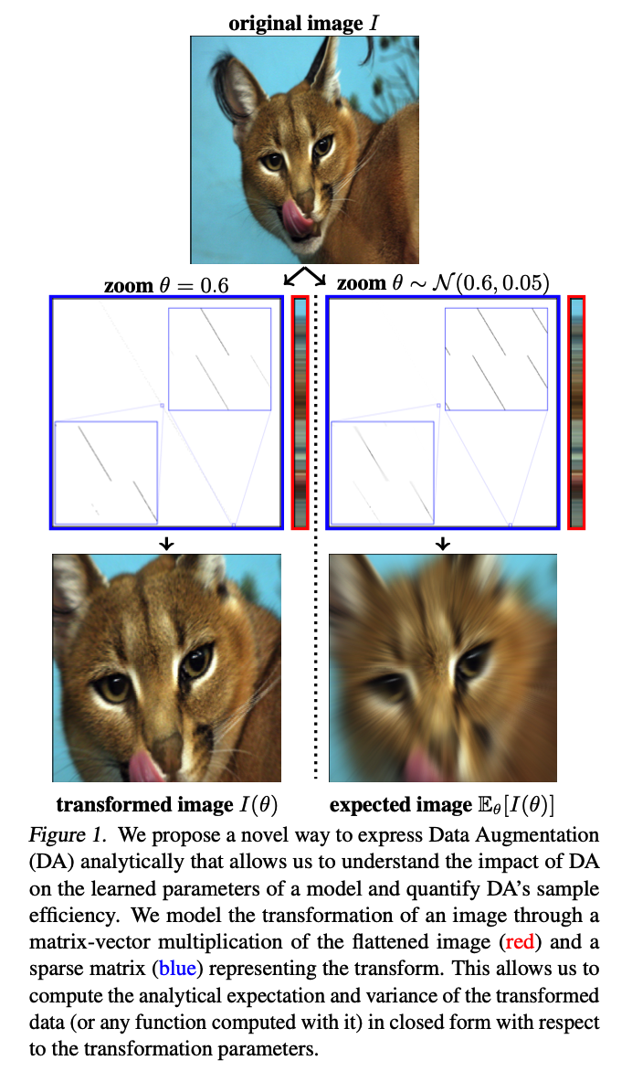
introduce Data-Space Transform (DST)

Contributions

• (a) derive the analytical first order moments of augmented samples & the losses employing augmented samples
  • effectively provide the explicit regularizer induced by each DA

• (b) quantify the number of DA samples that are required for a model/loss to obtain a correct estimate of the information conveyed by that DA

• (c) derive the sensitivity of a given loss and model under a DA policy
  • TangentProp : natural regularization to employ to minimize the loss variance

2. Background

(1) Explicit Regularizers From DA

DA regularizes a model towards the transformations

Estimate the impact of DA onto \(f_\gamma\),

• derive the explicit regularizer that directly acts upon \(f_\gamma\) in the same manner as if one were to use DA during training
• This explicit derivation is however challenging
  • limited to “additive white noise” or “multiplicative binary noise”

Relationship between DA & weight decay

• (linear case)
  • \(\min _{\boldsymbol{W}} \sum_{n=1}^N \mathbb{E}_{\boldsymbol{\epsilon} \sim \mathcal{N}(0, \sigma)}\left[\left\|\boldsymbol{y}_n-\boldsymbol{W}(\boldsymbol{x}+\boldsymbol{\epsilon})\right\|_2^2\right]= \min _{\boldsymbol{W}} \sum_{n=1}^N\left\|\boldsymbol{y}_n-\boldsymbol{W} \boldsymbol{x}\right\|_2^2+\lambda(\sigma)\|\boldsymbol{W}\|_F^2\).
• (nonlinear case)
  • DA = adding an explicit Frobenius norm regularization onto the Jacobian of \(f_\theta\) evaluated at each data sample.

Advanced case

• weight-decay \(\neq\) “more advanced DA”

• norm-based regularization : insufficient to describe the implicit regularization of DAs ( involving advanced image transformations )

(2) Coordinate Space Transformation

• consider a 2D-image \(I(x, y)\) at least square-integrable \(I \in L^2\left(\mathbb{R}^2\right)\)

• Multi-channel images : by applying the same transformation on each channel
• assume that \(I\) has compact support
  • e.g. has nonzero values only within a bounded domain such as \([0,1]^2\).

Most common formulation to apply a transformation on the image \(I\)

= transform the image coordinates

= mapping \(t: \mathbb{R}^2 \mapsto \mathbb{R}^2\) …. \(T(u, v)=I(t(u, v))\)

Function \(t\) : often has some parameter \(\theta\)

\(\begin{aligned} & t_\theta(x, y)=\left[x-\theta_1, y-\theta_2\right]^T, \quad \text { (translation) } \\ & t_\theta(x, y)=\left[\begin{array}{cc} \cos (\theta) & -\sin (\theta) \\ \sin (\theta) & \cos (\theta) \end{array}\right]\left[\begin{array}{l} x \\ y \end{array}\right], \quad \text { (rotation) } \\ & t_\theta(x, y)=\left[\theta_1 x, \theta_2 y\right]^T, \quad \text { (zoom) } \\ & \end{aligned}\).

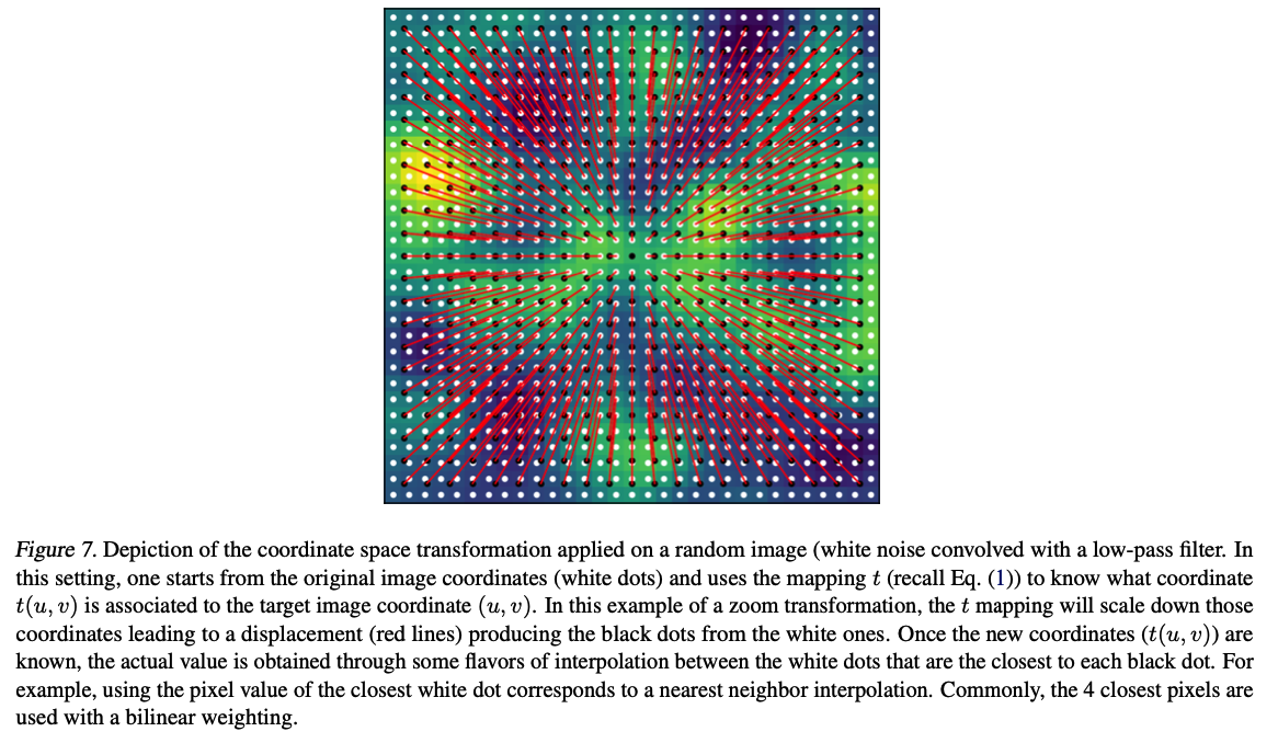
BENEFITS of formulation as \(T(u, v)=I(t(u, v))\) :

• (1) allows a simple and intuitive design of \(t\) to obtain novel transformations
• (2) computationally efficient
  • \(\because\) coordinate-space of images are 2/3-D

\(\rightarrow\) led to the design of DNN architecture with explicit coordinate transformations

DRAWBACKS of formulation as \(T(u, v)=I(t(u, v))\) :

• (1) computing the “exact moments” of the transformed image under random \(\theta\) parameters (e.g. the expectation \(\mathbb{E}_\theta\left[I \circ t_\theta\right]\) ) is not tractable
  • \(\because\) composition of \(t\) with the nonlinear mapping \(I\)

\(\rightarrow\) computing such quantities is crucial !!!

• to understand many properties around the use of DA sampling during training
  • e.g. to study its impact onto a model’s parameters.

3. Analytical Moments of Transformed Images Enable Infinite Dataset Training

Overview

(Section 3.1)

• training process under DA sampling

  = doing a Monte-Carlo estimate of the true (unknown) expected loss under DA distn

(Section 3.2)

• expectation and variance of a transformed sample
• construction of a novel Data-Space Transformation (DTS)

(Section 3.3)

• closed-form formula of those moments

(Section 3.4)

• remove the need to sample transformed images to train a model,

  ( by obtaining the closed-form expected loss )

(1) Motivation: Current Data-Augmentation Training Performs Monte-Carlo Estimation

Training a model with DA :

• (i) sampling transformed images
  • for each sample \(\boldsymbol{x}_n\) as in \(\mathcal{T}_{\theta_n}\left(\boldsymbol{x}_n\right)\) with \(\theta_n \sim \boldsymbol{\theta}\)
• (ii) evaluating the loss \(\mathcal{L}\) on the transformed data
• (iii) update the parameters \(\gamma\) of the model \(f_\gamma\).

\(\rightarrow\) corresponds to a one-sample Monte Carlo (MC) estimate

(Metropolis et al., 1953; Hastings, 1970) of the expected loss

• \(\sum_{n=1}^N \mathbb{E}_{\boldsymbol{\theta}}\left[\mathcal { L } ( f _ { \gamma } ( \mathcal { T } _ { \boldsymbol { \theta } } ( \boldsymbol { x } _ { n } ) ) \right] \approx \sum _ { n = 1 } ^ { N } \mathcal { L } \left(f_\gamma\left(\mathcal{T}_{\theta_n}\left(\boldsymbol{x}_n\right)\right) \right.\).
  • where \(\theta_n \sim \boldsymbol { \theta }\).

One-sample estimate : insufficient to apply CLT

\(\leftrightarrow\) combination of multiple samples in each mini-batch & repeated i.i.d sampling

\(\rightarrow\) provide convergence in most cases

Example) SSL loss : heavily rely on DA

• tend to diverge if the mini-batch size is not large enough

  ( as opposed to supervised losses )

• To avoid such instabilities

  \(\rightarrow\) compute the model parameters’ gradient on the expected loss

Closed-form expected loss requires knowledge of the expectation and variance of the transformed sample \(\mathcal{T}_{\boldsymbol{\theta}}\left(\boldsymbol{x}_n\right)\)

\(\rightarrow\) \(\therefore\) propose to formulate a novel and tractable augmentation model

(2) Proposed Data-Space Transformation

9 Instead of altering the coordinate positions of an image )

\(\rightarrow\) propose to alter the image basis functions

any (image) function can be expanded into its basis as in

• \(I(u, v)=\int I(x, y) \delta(u-x, v-y) d x d y\).
  • \(\delta\) : Dirac distn

Ex) horizontal translation ( by a constant \(\theta\) )

• \(T(u, v)=\int I(x, y) \delta(u-x-\theta, v-y) d x d y\).

  • moving the basis functions onto which the image is evaluated

    ( rather than by moving the image’s coordinate )

\(\rightarrow\) derivation of the transformed images expectation and variance, under random \(\theta\), will become straightforward

\(\rightarrow\) coin this transform as Data-Space Transform (DST)

Data-Space Transform

DST of an image \(I \in L^2\left(\mathbb{R}^2\right)\)

= producing the transformed image \(T \in L^2\left(\mathbb{R}^2\right)\) as

• \(T(u, v)=\int I(x, y) h_\theta(u, v, x, y) d x d y\).
  • with \(h_\theta(u, v, .,.) \in \mathbb{C}_0^{\infty}\left(\mathbb{R}^2\right)\) encoding the transformation.

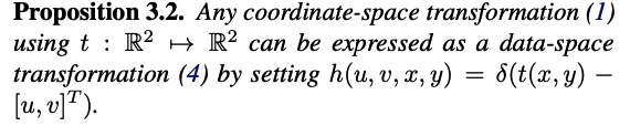
Coordinate-spcae transformations as DSTs

( Coordinate-space transformation = CST )

CST & DST act in different spaces

• CST : acts in the image input space
• DST: acts in the image output space

\(\rightarrow\) Does not limit the range of transformations that can be applied to an image

Examples) \(h_\theta(u, v, x, y)\)

1. Vertical/Horizontal translation
   • \(\delta\left(u-x+\theta_1, v-y+\theta_2\right)\).
2. Vertical/Horizontal shearing
   • \(\delta\left(u-x-\theta_1 y, v-y-\theta_2 x\right)\).
3. Zoom
   • \(\delta(u-\theta x, v-\theta y)\).
4. Rotation
   • \(\delta(u-\cos (\theta) x+\sin (\theta) y, v-\sin (\theta) x-\cos (\theta) y)\).

Before focusing on the analytical moments of the DST samples …

we describe how those operators are applied in a discrete setting.

Discretized version

\(\boldsymbol{x} \in \mathbb{R}^{h w}\) : flattend \((h \times w)\) discrete images \(I\)

DST ( with param \(\theta\) ) : \(\boldsymbol{t}(\theta)=\boldsymbol{M}(\theta) \boldsymbol{x}\)

• \(\boldsymbol{t}(\theta) \in \mathbb{R}^{h w}\) : flattened transformed image
• \(\boldsymbol{M}(\theta) \in \mathbb{R}^{h w \times h w}\) : matrix whose rows encode the discrete and flattened \(h_\theta(u, v, .,\).)

Ex) Zoom

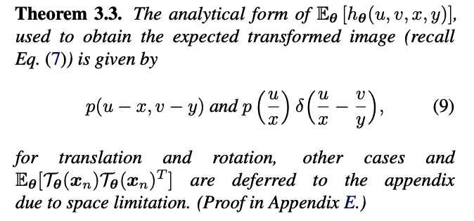
(3) Analytical Expectation and Variance of Transformed Images

DST : \(T(u, v)=\int I(x, y) h_\theta(u, v, x, y) d x d y\)

\(\rightarrow\) make the analytical form of the first two moments of an augmented sample straightforward to derive

Propose a step-by-step derivation of \(\mathbb{E}_{\boldsymbol{\theta}}\left[\mathcal{T}_{\boldsymbol{\theta}}(I)\right]\)

• ex) horizontal translation

  \(T(u, v)=\int I(x, y) \delta(u-x-\theta, v-y) d x d y\).

(1) Fubini’s theorem

• to switch the order of integration
• \(\mathbb{E}_{\boldsymbol{\theta}}\left[\mathcal{T}_{\boldsymbol{\theta}}(I)(u, v)\right]=\int I(x, y) \mathbb{E}_{\boldsymbol{\theta}}\left[h_{\boldsymbol{\theta}}(u, v, x, y)\right] d x d y\).

(2) Translation : \(\delta\left(u-x+\theta_1, v-y+\theta_2\right)\)

• \(\begin{aligned} \mathbb{E}_{\boldsymbol{\theta}}[\delta(u-x-\theta, v-y)] & =\int \delta(u-x-\theta, v-y) p(\theta) d \theta \\ & =p(u-x) \delta(v-y), \end{aligned}\).
  • \(p\) : density function of \(\boldsymbol{\theta}\)

(3) Expected augmented image at coordinate \((u, v)\) :

• \(\begin{aligned} \mathbb{E}_{\boldsymbol{\theta}}\left[\mathcal{T}_{\boldsymbol{\theta}}(I)(u, v)\right] & =\int I(x, y) p(u-x) \delta(v-y) d x d y \\ & =\int I(x, v) p(u-x) d x \end{aligned}\).

• further simplified into \(\mathbb{E}_{\boldsymbol{\theta}}\left[\mathcal{T}_{\boldsymbol{\theta}}(I)(., v)\right]=\) \(I(., v) \star p\).

\(\therefore\) Expected translated image

= convolution (on the \(x\)-axis only) between the original image \(I\) & univariate density function \(p\).

Discretized version of the expected image

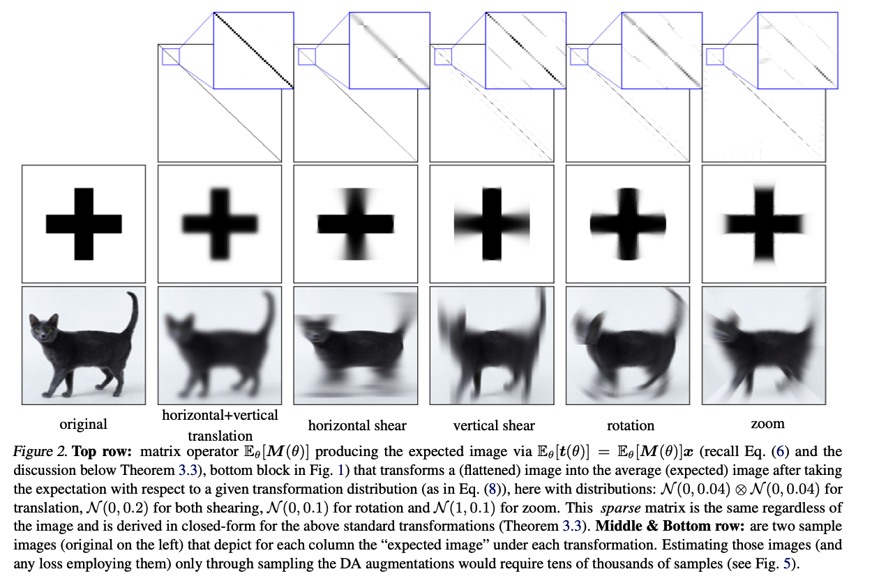
• \(\mathbb{E}_{\boldsymbol{\theta}}[\boldsymbol{t}(\boldsymbol{\theta})]=\mathbb{E}_{\boldsymbol{\theta}}[\boldsymbol{M}(\boldsymbol{\theta})] \boldsymbol{x}\) ,

  with the entries of \(\mathbb{E}_{\boldsymbol{\theta}}[\boldsymbol{M}(\boldsymbol{\theta})]\) given by discretizing \(p(u-x, v-y) \text { and } p\left(\frac{u}{x}\right) \delta\left(\frac{u}{x}-\frac{v}{y}\right)\).

(4) The Explicit Regularizer of Data-Augmentations

Settings : LR model with MSE loss function

Expected loss under DA sampling :

\[\sum_{n=1}^N \mathbb{E}_{\boldsymbol{\theta}}\left[\mathcal { L } ( f _ { \gamma } ( \mathcal { T } _ { \boldsymbol { \theta } } ( \boldsymbol { x } _ { n } ) ) \right] \approx \sum _ { n = 1 } ^ { N } \mathcal { L } \left(f_\gamma\left(\mathcal{T}_{\theta_n}\left(\boldsymbol{x}_n\right)\right) \right.\]

\(\rightarrow\) \(\mathcal{L}=\sum_{n=1}^N \mathbb{E}_{\boldsymbol{\theta}}\left[\left\|\boldsymbol{y}_n-\boldsymbol{W} \mathcal{T}_{\boldsymbol{\theta}}\left(\boldsymbol{x}_n\right)-\boldsymbol{b}\right\|_2^2\right]\)

• \(\boldsymbol{x}_n \in \mathbb{R}^D, n=1, \ldots, N\) : input (flattened) \(\mathrm{n}^{\mathrm{th}}\) image \(I_n\)

• \(\boldsymbol{y}_n \in \mathbb{R}^K\) : the \(\mathrm{n}^{\text {th }}\) target vector
• \(\boldsymbol{W} \in\) \(\mathbb{R}^{K \times D}, \boldsymbol{b} \in \mathbb{R}^K\) the model’s parameters

Derive the exact loss of above, as a function of the sample mean and variance

• drop \(\theta\) subscript for clarity

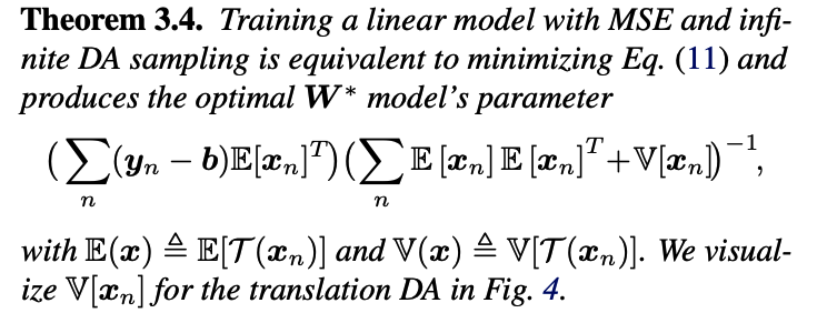
• \(\sum_{n=1}^N\left\|\boldsymbol{y}_n-\boldsymbol{W} \mathbb{E}\left[\mathcal{T}\left(\boldsymbol{x}_n\right)\right]-\boldsymbol{b}\right\|_2^2+\left\|\boldsymbol{W} \boldsymbol{Q}(\boldsymbol{x}) \Lambda(\boldsymbol{x})^{\frac{1}{2}}\right\|_F^2\).
  • spectral decomposition \(\boldsymbol{Q}(\boldsymbol{x}) \Lambda(\boldsymbol{x}) \boldsymbol{Q}(\boldsymbol{x})^T=\) \(\mathbb{V}[\mathcal{T}(\boldsymbol{x})]\).
• (term 2) explicit DA regularizer
  • pushes the kernel space of \(W\) to align with the largest principal directions of the data manifold tangent space
  • largest eigenvectors in \(\boldsymbol{Q}(\boldsymbol{x})\) : principal directions of the data manifold tangent space at \(\boldsymbol{x}\), as encoded via \(\mathbb{V}[\mathcal{T}(\boldsymbol{x})]\).

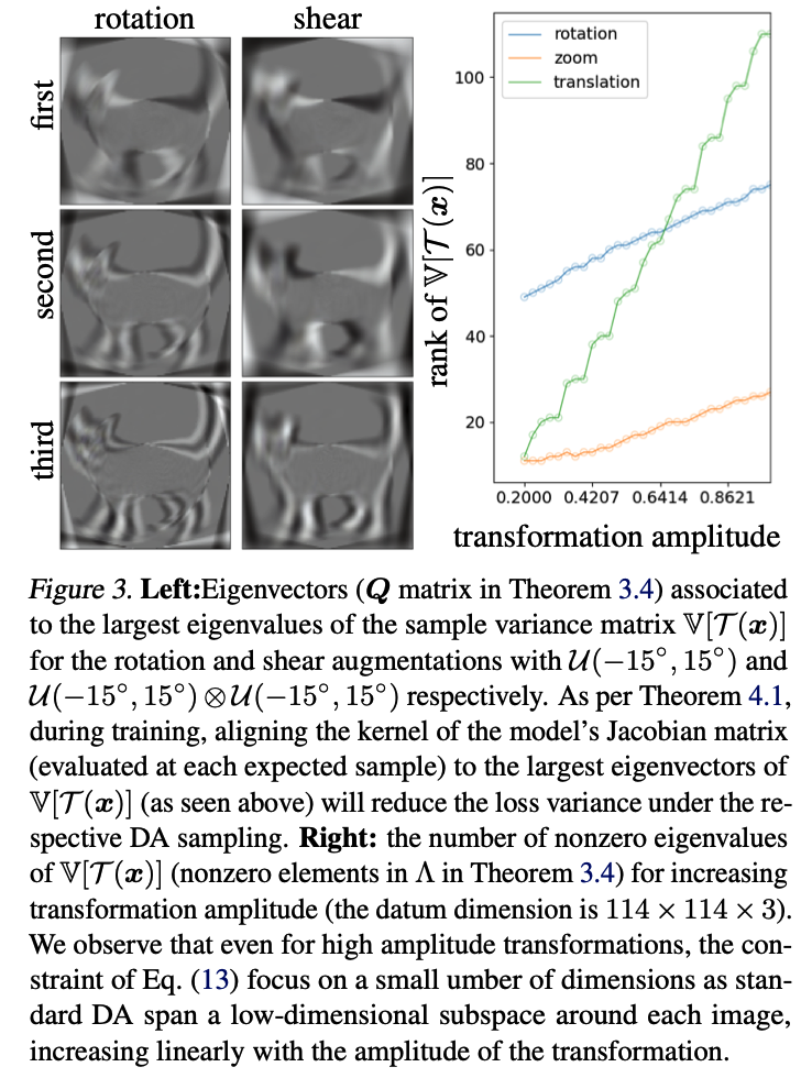
• visualization of \(Q\) and \(\Lambda\) for different DAs,
• show how each DA policy impacts the model’s parameter \(W\) through the regularization

The knowledge of \(\mathbb{E}[\mathcal{T}(\boldsymbol{x})]\) and \(\mathbb{V}[\mathcal{T}(\boldsymbol{x})]\) enables to train a LR model on the true expected loss

( For NON-linear setting )

• use a truncated Taylor approximation of the nonlinear model
• same regularization (as above), but with the model’s Jacobian matrix \(\boldsymbol{J} f_\gamma\left(\boldsymbol{x}_n\right)\) in-place of \(\boldsymbol{W}\)