(paper 40) GraphCL

Graph Contrastive Learning with Augmentations

Contents

1. Abstract
2. Introduction
3. Related Work
   1. GNN
4. Methodology
   1. Data Augmentation for Graphs
   2. Graph Contrastive Learning

0. Abstract

SSL & pretraining : less explored for GNNs

propose graph contrastive learning (GraphCL)

• for learning unsupervised representations of graph data

Details

• design four types of graph augmentations
• study the impact of various combinations of graph augmentations on multiple datasets, in four different settings :
  • semi-supervised
  • unsupervised
  • transfer learning
  • adversarial attacks

1. Introduction

Graph neural networks (GNNs)

• neighborhood aggregation scheme
• various tasks
  • ex) node/link/graph classification, link prediction, graph classification
• little exploration of (self-supervised) pre-training

This paper : argue for the necessity of exploring GNN pre-training schemes

( naïve approach : ( for graph-level task ) reconstruct the vertex adjacency information )

Contribution

• propose a novel graph contrastive learning framework (GraphCL) for GNN pre-training

• design 4 types of graph data augmentations,

  ( each of which imposes certain prior over graph data and parameterized for the extent and pattern )

2. Related Work

(1) GNN

Idea : iterative neighborhood aggregation (or message passing) scheme

Notation

• \(\mathcal{G}=\{\mathcal{V}, \mathcal{E}\}\) : undirected graph

  • \(\boldsymbol{X} \in \mathbb{R}^{\mid \mathcal{V} \mid \times N}\) : feature matrix
    • \(\boldsymbol{x}_n=\boldsymbol{X}[n,:]^T\) : \(N\)-dim attribute vector of node \(v_n \in \mathcal{V}\)

• \(f(\cdot)\) : K-layer GNN

• propagation of \(k\)th layer :

  • step 1) \(\boldsymbol{a}_n^{(k)}=\operatorname{AGGREGATION}^{(k)}\left(\left\{\boldsymbol{h}_{n^{\prime}}^{(k-1)}: n^{\prime} \in \mathcal{N}(n)\right\}\right)\)

  • step 2) \(\boldsymbol{h}_n^{(k)}=\operatorname{COMBINE}^{(k)}\left(\boldsymbol{h}_n^{(k-1)}, \boldsymbol{a}_n^{(k)}\right)\)

    ( = embedding of vertex \(v_n\) at \(k\)th layer, where \(\boldsymbol{h}_n^{(0)}=\boldsymbol{x}_n\) )

• \(\mathcal{N}(n)\) : set of vertices adjacent to \(v_n\)

After the \(K\)-layer propagation….

\(\rightarrow\) output embedding for \(\mathcal{G}\) : summarized on layer embeddings, with READOUT function

( + MLP for downstream task )

• step 3) \(f(\mathcal{G})=\operatorname{READOUT}\left(\left\{\boldsymbol{h}_n^{(k)}: v_n \in \mathcal{V}, k \in K\right\}\right)\)
• step 4) \(\boldsymbol{z}_{\mathcal{G}}=\operatorname{MLP}(f(\mathcal{G}))\)

3. Methodology

(1) Data Augmentation for Graphs

focus on graph-level augmentations

• given a graph datasets \(\mathcal{G} \in\left\{\mathcal{G}_m: m \in M\right\}\) ( = consists of \(M\) graphs )

  \(\rightarrow\) augmented graph : \(\hat{\mathcal{G}} \sim q(\hat{\mathcal{G}} \mid \mathcal{G})\)

  ( augmentation distribution, conditioned on the original graph )

focus on 3 categories :

• (1) biochemical molecules
• (2) social networks
• (3) image super-pixel graphs

propose 4 general DA for graph-structured data

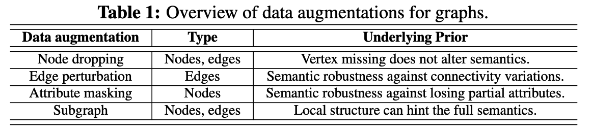
a) Node Dropping

• randomly discard certain portion of vertices ( along with their connections )
• node’s dropping probability : i.i.d. uniform distn

b) Edge Perturbation

• perturb the connectivities in graph

  ( by randomly adding / dropping certain ratio of edges )

• edge add/drop probability : i.i.d. uniform distn

c) Attribute Masking

• prompts models to recover masked vertex attributes using their context information ( remaining attributes )

d) Subgraph

• samples a subgraph from \(G\) using random walk

(2) Graph Contrastive Learning

propose a graph contrastive learning framework (GraphCL) for (self-supervised) pre-training of GNNs

Graph CL : performed through maximizing the agreement between two augmented views of the same graph via a contrastive loss

4 major components

• (1) Graph data augmentation \(q_i(\cdot \mid \mathcal{G})\)

  • \(\hat{\mathcal{G}}_i \sim q_i(\cdot \mid \mathcal{G}), \hat{\mathcal{G}}_j \sim q_j(\cdot \mid \mathcal{G})\).
  • for different domains of graph datasets, select appropriate DA strategy

• (2) GNN-based encoder \(f(\cdot)\)

  • extracts graph-level representation vectors \(\boldsymbol{h}_i, \boldsymbol{h}_j\) ( for augmented graphs \(\hat{\mathcal{G}}_i, \hat{\mathcal{G}}_j\) )

• (3) Projection head \(g(\cdot)\)

  • non-linear transformation

  • map to latent space where the contrastive loss is calculated

    ( obtain \(\boldsymbol{z}_i, \boldsymbol{z}_j\) )

  • ex) in GCL : 2-layer MLP

• (4) Contrastive loss function \(\mathcal{L}(\cdot)\)

  • enforce maximizing the consistency between positive pairs \(\boldsymbol{z}_i, \boldsymbol{z}_j\) compared with negative pairs
  • use NT-Xent ( = normalized temperature-scaled cross entropy loss )
    • \(\ell_n=-\log \frac{\exp \left(\operatorname{sim}\left(\boldsymbol{z}_{n, i}, \boldsymbol{z}_{n, j}\right) / \tau\right)}{\sum_{n^{\prime}=1, n^{\prime} \neq n}^N \exp \left(\operatorname{sim}\left(\boldsymbol{z}_{n, i}, \boldsymbol{z}_{n^{\prime}, j}\right) / \tau\right)}\).
      • ex) where \(\operatorname{sim}\left(\boldsymbol{z}_{n, i}, \boldsymbol{z}_{n, j}\right)=\boldsymbol{z}_{n, i}^{\top} \boldsymbol{z}_{n, j} / \mid \mid \boldsymbol{z}_{n, i} \mid \mid \mid \mid \boldsymbol{z}_{n, j} \mid \mid\)