(paper 49) VIME

VIME : Extending the Success of Self- and Semi-supervised Learning to Tabular Domain

Contents

1. Abstract
2. Introduction
3. Related Works
   1. Self-SL
   2. Semi-SL
4. Problem Formulation
   1. Self-SL
   2. Semi-SL
5. Proposed Model : VIME
   1. Self-SL for tabular data
   2. Semi-SL for tabular data

0. Abstract

Self- and semi-supervised learning :

• a lot of progress in NLP & CV

• heavily rely on the unique structure in the domain datasets

  • ex) NLP : semantic relationships in language
  • ex) CV : spatial relationships in images

  \(\rightarrow\) not adaptable to general tabular data

VIME (proposal)

( = Value Imputation and Mask Estimation )

• novel self- and semi-supervised learning for tabular data
• (1) create a novel “pretext task” :
  • estimating mask vectors from corrupted tabular data
• (2) introduce a novel “tabular data augmentation method”

1. Introduction

Scarce labeled datsets

• ex) 100,000 Genomes project
  • sequenced 100,000 genomes from around 85,000 NHS patients affected by a rare disease
  • rare diseases occur in 1 / 2000 people

No effective self / semi SL for tabular data

\(\because\) heavily rely on the spatial or semantic structure of image or language data

[ Self SL ] pretext tasks

• ex) ( NLP ) BERT : 4 different pretext tasks
• ex) ( CV ) rotation, jigsaw puzzle, and colorization

[ Semi SL ] regularizer

• regularizers they use for the predictive model are based on some prior knowledge of these data structures

• ex) consistency regularizer :

  • encourages the predictive model to have the same output distribution on a sample and its augmented variants ( ex. rotation, convex combination of images )

    \(\rightarrow\) not applicable in Tabular data

Contribution

propose novel self /semi SL for tabular data

• (1) self SL : introduce a novel pretext task

  • mask vector estimation ( in addition to feature vector estimation )

• (2) semi SL : introduce a novel tabular DA

  • use the trained encoder to generate multiple augmented samples

    • by masking each data using several different masks

      & imputing the corrupted values for each masked data point

\(\rightarrow\) propose VIME (Value Imputation and Mask Estimation)

2. Related Works

(1) Self-SL

categorized into 2 types :

• (1) pretext task
• (2) contrastive learning

(1) pretext task

• mostly appropriate for images / natural language
• examples )
  • images ) surrogate classes prediction (scaling and translation), rotation degree predictions, colorization, relative position of patches estimation, jigsaw puzzle solving, image denoising, partial-to-partial registration
  • natural language ) next words and previous words predictions

(2) contrastive learning

• also mostly appropriate for images / natural language
• examples ) contrastive predictive coding, contrastive multi-view coding, SimCLR, momentum contrast

existing work on self-supervised learning, applied to tabular data

• DAE (Denoising Auto-Encoder)
  • pretext task : recover the original sample from a corrupted sample
• Context Encoder
  • pretext task : reconstruct the original sample from both the corrupted sample and the mask vector.
• TabNet, TaBERT
  • pretext task : recovering corrupted tabular data

[ Proposal ]

• new pretext task : recover the mask vector
• novel tabular data augmentation

(2) Semi-SL

categorized into 2 types :

• (1) entropy minimization
• (2) consistency regularization

(1) entropy minimization

• encourages a classifier to output low entropy predictions on unlabeled data

(2) consistency regularization

• encourages consistency between a data & stochastically altered version of data

• ex) Mean teacher, VAT

• ex) MixMatch, ReMixMatch = (1) + (2)

3. Problem Formulation

Notation

• \(\mathcal{D}_l=\left\{\mathbf{x}_i, y_i\right\}_{i=1}^{N_l}\) : (small) LABELED data
• \(\mathcal{D}_u=\left\{\mathbf{x}_i\right\}_{i=N_l+1}^{N_l+N_u}\) : (large) UNLABELED data
  • where \(N_u \gg N_l, \mathbf{x}_i \in \mathcal{X} \subseteq \mathbb{R}^d\)
  • where \(N_u \gg N_l, \mathbf{x}_i \in \mathcal{X} \subseteq \mathbb{R}^d\) & \(y_i \in \mathcal{Y}\)
    • \(y_i\) : scalar / multi-dim vector
      • scalar ( in single-task learning )
      • multi-dim vector ( in multi-task learning )
• \(f: \mathcal{X} \rightarrow \mathcal{Y}\) : predictive model
• Loss
  • \(\sum_{i=1}^{N_l} l\left(f\left(\mathbf{x}_i\right), y_i\right)\) : empirical supervised loss
  • \(\mathbb{E}_{(\mathbf{x}, y) \sim p_{X, Y}}[l(f(\mathbf{x}), y)]\) : expected supervised loss

Assumption :

• \(\mathbf{x}_i\) in \(\mathcal{D}_l\) and \(\mathcal{D}_u\) is sampled i.i.d. from a feature distribution \(p_X\)
• \(\left(\mathbf{x}_i, y_i\right)\) in \(\mathcal{D}_l\) are drawn from a joint distribution \(p_{X, Y}\)
  • only limited labeled samples from \(p_{X, Y}\) are available

(1) Self-SL

focus on pretext tasks

• challenging, but highly relevant to the downstream tasks that we attempt to solve

self-supervised learning

• (1) encoder function \(e: \mathcal{X} \rightarrow \mathcal{Z}\)

  • input : \(\mathbf{x} \in \mathcal{X}\)
  • output : \(\mathbf{z}=e(\mathbf{x}) \in \mathcal{Z}\)
    • \(\mathbf{z}\) is optimized to solve a pretext task,
      • defined with (1) pseudo-label \(y_s \in \mathcal{Y}_s\) & (2) self-supervised loss function \(l_{s s}\)

• (2) pretext predictive model : \(h: \mathcal{Z} \rightarrow \mathcal{Y}_s\)

  • trained jointly with the encoder function \(e\) ,

    by minimizing the expected self-supervised loss function \(l_{s s}\)

    ( \(\min _{e, h} \mathbb{E}_{\left(\mathbf{x}_s, y_s\right) \sim p_{X_s, Y_s}}\left[l_{s s}\left(y_s,(h \circ e)\left(\mathbf{x}_s\right)\right)\right]\) )

(2) Semi-SL

optimizes the predictive model \(f\) , by minimizing (1) + (2)

• (1) supervised loss function
• (2) unsupervised loss function

\(\min _f \mathbb{E}_{(\mathbf{x}, y) \sim p_{X Y}}[l(y, f(\mathbf{x}))]+\beta \cdot \mathbb{E}_{\mathbf{x} \sim p_X, \mathbf{x}^{\prime} \sim \tilde{p}_X\left(\mathbf{x}^{\prime} \mid \mathbf{x}\right)}\left[l_u\left(f(\mathbf{x}), f\left(\mathbf{x}^{\prime}\right)\right)\right]\).

• \(\mathbf{x}^{\prime}\) : perturbed version of \(\mathbf{x}\)
  • assumed to be drawn from a conditional distribution \(\tilde{p}_X\left(\mathbf{x}^{\prime} \mid \mathbf{x}\right)\)
• term (1) : estimated using \(\mathcal{D}_l\)
• term (2) : estimated using \(\mathcal{D}_u\)

4. Proposed Model: VIME

(1) Self-SL : propose two pretext tasks

(2) Semi-SL : develop an unsupervised loss function

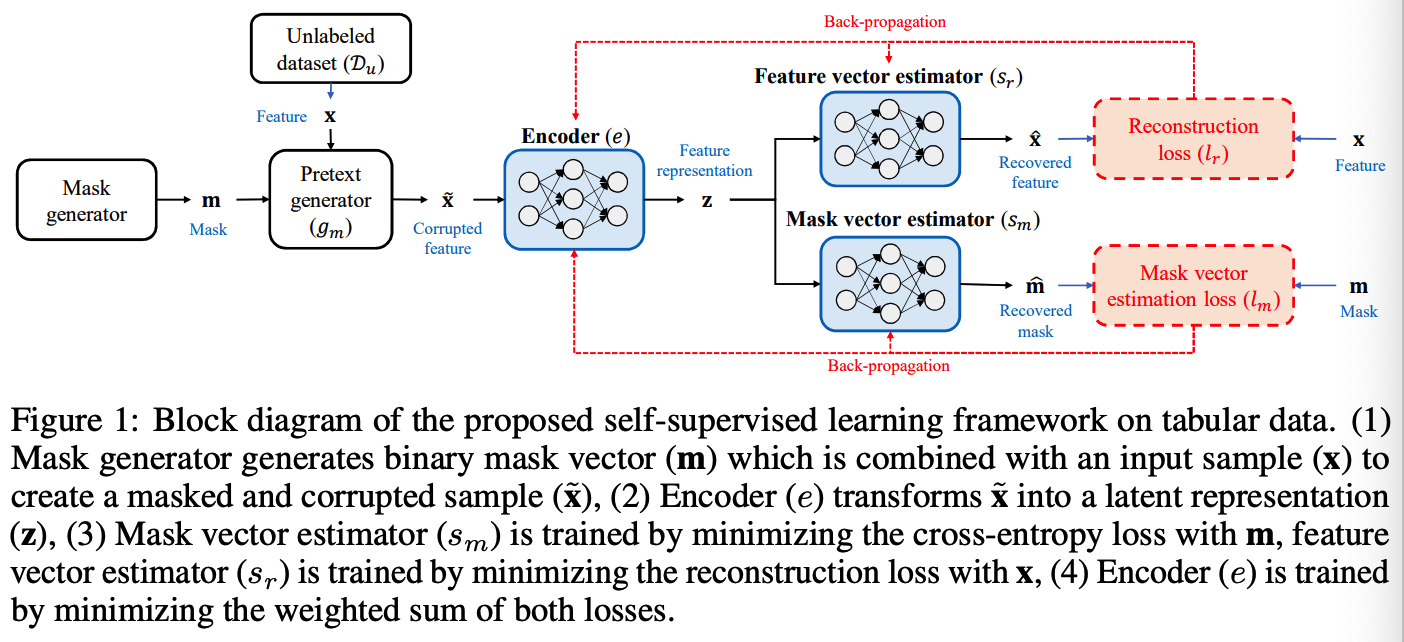
(1) Self-SL for tabular data

propose 2 pretext tasks :

• (1) feature vector estimation
• (2) mask vector estimation.

Goal : optimize a pretext model to….

• recover an input sample (a feature vector) from its corrupted variant,
• estimate the mask vector that has been applied

Notation

• pretext distribution : \(p_{X_s, Y_s}\)

• binary mask vector : \(\mathbf{m}=\left[m_1, \ldots, m_d\right]^{\top} \in\{0,1\}^d\)

  • \(m_j\) : randomly sampled from a Bernoulli distribution with prob \(p_m\)

    ( \(p_{\mathbf{m}}=\prod_{j=1}^d \operatorname{Bern}\left(m_j \mid p_m\right)\) )

• pretext generator : \(g_m: \mathcal{X} \times\{0,1\}^d \rightarrow \mathcal{X}\)

  • input : \(\mathbf{x}\) from \(\mathcal{D}_u\) & mask vector \(\mathbf{m}\)
  • output : masked sample \(\tilde{\mathbf{x}}\)

Pretext Generation

\(\tilde{\mathbf{x}}=g_m(\mathbf{x}, \mathbf{m})=\mathbf{m} \odot \overline{\mathbf{x}}+(1-\mathbf{m}) \odot \mathbf{x}\).

• where the \(j\)-th feature of \(\overline{\mathbf{x}}\) is sampled from the empirical distribution \(\hat{p}_{X_j}=\frac{1}{N_u} \sum_{i=N_l+1}^{N_l+N_u} \delta\left(x_j=\right.\) \(x_{i, j}\) )
  • where \(x_{i, j}\) is the \(j\)-th feature of the \(i\)-th sample in \(\mathcal{D}_u\)
• corrupted sample \(\tilde{\mathbf{x}}\) is not only tabular but also similar to the samples in \(\mathcal{D}_u\)
• (compared to Gaussian Noise, etc … )
  • generates \(\tilde{\mathbf{x}}\) that is more difficult to distinguish from \(\mathbf{x}\)

Two randomness

( in pretext distribution \(p_{X_s, Y_s}\) )

• (1) \(\mathbf{m}\) : random vector ( randomness from Bernoulli distn )
• (2) \(g_m\) : pretext generator ( randomness from \(\overline{\mathbf{x}}\) )

\(\rightarrow\) increases the difficulty of reconstruction

( difficulty can be adjusted by hyperparameter \(p_m\) ( = prob of corruption) )

Compared to conventional methods, more challenging

( conventional methods ex : rotation, coloring… )

• (conventional) just correcting the raw value
• (proposed masking) completely removes some of the features from \(\mathbf{x}\) & replaces them with a noise sample \(\overline{\mathbf{x}}\) , which each feature may come from a different random sample in \(\mathcal{D}_u\)

Divide the task into 2 sub-tasks ( = pretext tasks )

• (1) Mask vector estimation : predict which features have been masked
• (2) Feature vector estimation : predict the values of the features that have been corrupted.

Predictive model

Separate pretext predictive model ( for each pretext task )

• (1) Mask vector estimator, \(s_m: \mathcal{Z} \rightarrow[0,1]^d\)
• (2) Feature vector estimator, \(s_r: \mathcal{Z} \rightarrow \mathcal{X}\)

Loss Function

\(\min _{e, s_m, s_r} \mathbb{E}_{\mathbf{x} \sim p_X, \mathbf{m} \sim p_{\mathbf{m}}, \tilde{\mathbf{x}} \sim g_m(\mathbf{x}, \mathbf{m})}\left[l_m(\mathbf{m}, \hat{\mathbf{m}})+\alpha \cdot l_r(\mathbf{x}, \hat{\mathbf{x}})\right]\).

• \(\hat{\mathbf{m}}=\left(s_m \circ e\right)(\tilde{\mathbf{x}})\) , \(\hat{\mathbf{x}}=\left(s_r \circ e\right)(\tilde{\mathbf{x}})\)

Term 1) \(l_m\) : sum of the BCE for each dimension of the mask vector

• \(l_m(\mathbf{m}, \hat{\mathbf{m}})=-\frac{1}{d}\left[\sum_{j=1}^d m_j \log \left[\left(s_m \circ e\right)_j(\tilde{\mathbf{x}})\right]+\left(1-m_j\right) \log \left[1-\left(s_m \circ e\right)_j(\tilde{\mathbf{x}})\right]\right],\).

Term 2) \(l_r\) : reconstruction loss

• \(l_r(\mathbf{x}, \hat{\mathbf{x}})=\frac{1}{d}\left[\sum_{j=1}^d\left(x_j-\left(s_r \circ e\right)_j(\tilde{\mathbf{x}})\right)^2\right]\).
• ( for categorical variables, modified with CE loss )

Intuition

• important for \(e\) to capture the correlation among the features of \(x\)

• \(s_m\) : identify the masked features from the inconsistency between feature values

• \(s_r\) : impute the masked features by learning from the correlated non-masked features

• ex) if the value of a feature is very different from its correlated features,

  \(\rightarrow\) this feature is likely masked and corrupted

(2) Semi-SL for tabular data

show how the encoder \(e\) can be used in semi-supervised learning

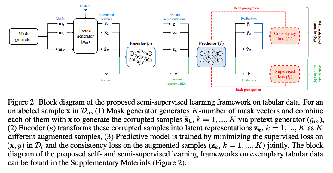
( \(f_e=f \circ e\) , \(\hat{y}=f_e(\mathbf{x})\) )

Train predictive model \(f\), with loss function below :

\(\mathcal{L}_{\text {final }}=\mathcal{L}_s+\beta \cdot \mathcal{L}_u\),

• ( supervised loss ) \(\mathcal{L}_s\)
  • \(\mathcal{L}_s=\mathbb{E}_{(\mathbf{x}, y) \sim p_{X Y}}\left[l_s\left(y, f_e(\mathbf{x})\right)\right]\).
  • ex) MSE, CE
• ( unsupervised (consistency) loss ) \(\mathcal{L}_u\)
  • \(\mathcal{L}_u=\mathbb{E}_{\mathbf{x} \sim p_X, \mathbf{m} \sim p_{\mathrm{m}}, \tilde{\mathbf{x}} \sim g_m(\mathbf{x}, \mathbf{m})}\left[\left(f_e(\tilde{\mathbf{x}})-f_e(\mathbf{x})\right)^2\right]\).
  • ( inspired by the idea in consistency regularizer )

stochastic approximation of \(\mathcal{L}_u\) :

• with \(K\) augmented samples
• \(\hat{\mathcal{L}}_u=\frac{1}{N_b K} \sum_{i=1}^{N_b} \sum_{k=1}^K\left[\left(f_e\left(\tilde{\mathbf{x}}_{i, k}\right)-f_e\left(\mathbf{x}_i\right)\right)^2\right]=\frac{1}{N_b K} \sum_{i=1}^{N_b} \sum_{k=1}^K\left[\left(f\left(\mathbf{z}_{i, k}\right)-f\left(\mathbf{z}_i\right)\right)^2\right]\).
  • \(N_b\) : batch size

output for a new test sample \(\mathbf{x}^t\) : \(\hat{y}=f_e\left(\mathbf{x}^t\right)\)