
Self-Supervised TS Representation Learning by Inter-Intra Relational Reasoning
Contents
- Abstract
- Introduction
- Method
- Inter-Sample relation reasoning
- Intra-Temporal relation reasoning
- Summary
0. Abstract
Most of traditional SSL :
-
focus on exploring the inter-sample structure
-
less efforts on the underlying intra-temporal structure
\(\rightarrow\) important for TS data
Self-Time
a general SSL TS representation learning framework
- explore the inter-sample relation and intra-temporal relation of TS
- learn the underlying structure feature on the unlabeled TS
Details :
- step 1-1) generate the inter-sample relation
- by sampling “pos & neg“ of anchor sample
- step 1-2) generate the intra-temporal relation
- by sampling “time pieces“ from this anchor sample
- step 2) feature extraction
- shared feature extraction backbone combined with two separate relation reasoning heads
- quantify the …
- (1) relationships of the “sample pairs” for inter-sample relation reasoning
- (2) relationships of the “time piece pairs” for intra-temporal relation reasoning
- step 3) useful representations of TS are extracted
1. Introduction
SSL in TS domain
- ex) metric learning based :
- triplet loss (Franceschi et al., 2019)
- contrastive loss (Schneider et al., 2019; Saeed et al., 2020)
- ex) multi-task learning based :
- predict different handcrafted features (Pascual et al., 2019a; Ravanelli et al., 2020)
- predict different signal transformations (Saeed et al., 2019; Sarkar & Etemad, 2020)
\(\rightarrow\) few of those works consider the INTRA-temporal structure of time series
Designing an efficient pretext task ( in SSL for TS ) is still an open probelm!
This paper explores the (1) inter-sample relation reasoning and (2) intra-temporal relation reasoning of TS
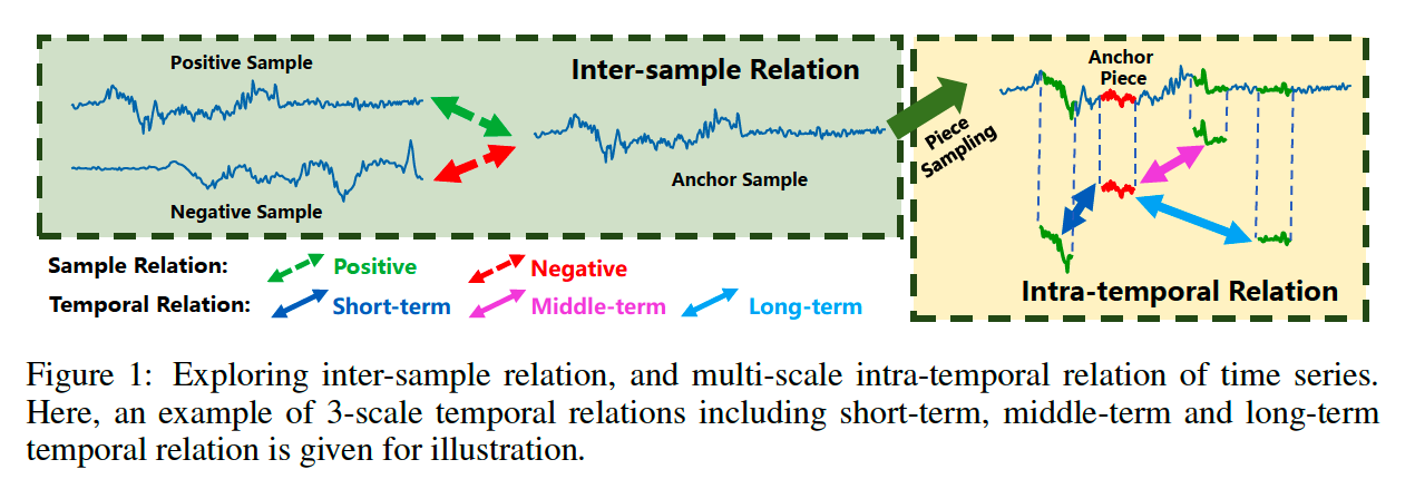
[ STEP 1-1 : inter-sample relation reasoning ]
- given an anchor sample, generate …
- pos : from its transformation counterpart
- neg : another individual sample
[ STEP 1-2 : intra-temporal relation reasoning ]
- (1) generate an anchor piece
- (2) sample several reference pieces
- to construct “different scales” of temporal relation ( between the anchor & reference )
- relation scales are determined based on the “temporal distance”
[ Step 2 & 3 ]
- step 2) shared feature extraction backbone quantifies the…
- (1) relationships between the sample pairs ( for inter-sample relation )
- (2) relationships between the time piece pairs ( for intra-temporal relation )
- step 3) extract useful representations of TS
Contribution
-
general self-supervised TS representation learning framework
- by investigating different levels of relations of time series data
- including inter-sample relation and intra-temporal relation
- by investigating different levels of relations of time series data
-
design a simple and effective intra-temporal relation sampling strategy
- to capture the underlying temporal patterns of TS
-
experiments on different categories of real-world time series data
& study the impact of different data augmentation strategies and temporal relation sampling strategies
2. Method
Notation
- Unlabeled TS : \(\mathcal{T}=\left\{\boldsymbol{t}_n\right\}_{n=1}^N\)
- each TS : \(\boldsymbol{t}_n=\left(t_{n, 1}, \ldots t_{n, T}\right)^{\mathrm{T}}\)
- Goal : learn a useful representation \(z_n=f_\theta\left(\boldsymbol{t}_n\right)\)
- from the backbone encoder \(f_\theta(\cdot)\)
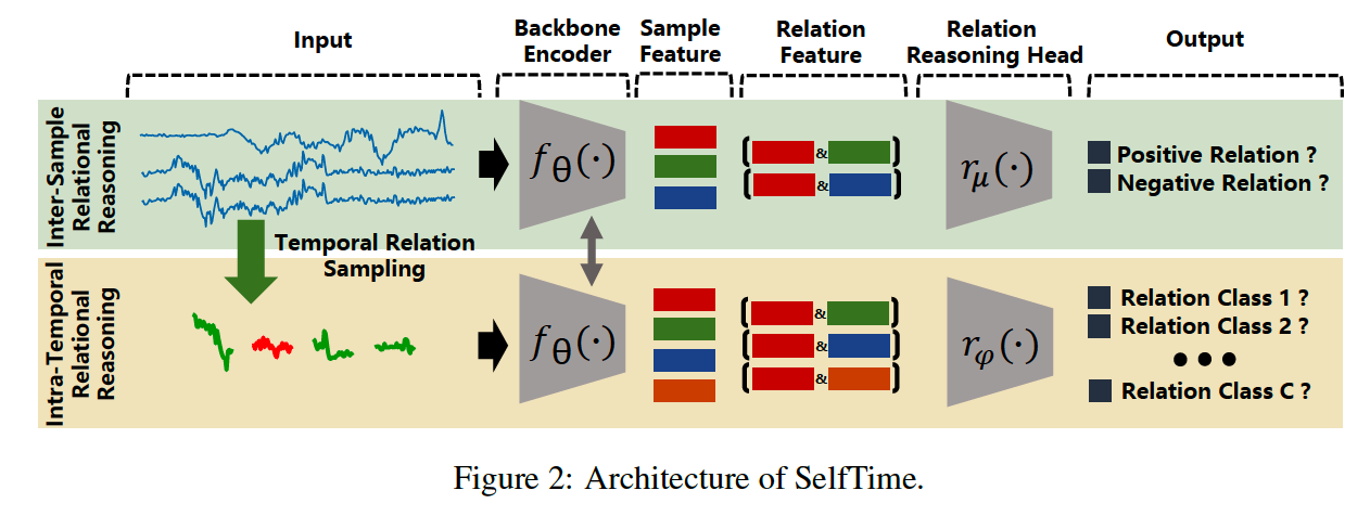
Consists of 2 branches
- (branch 1) inter-sample relational reasoning branch
- (branch 2) intra-temporal relational reasoning branch
Process
- Input : original TS & sampled time pieces
- Feature Extraction
- Extracts TS feature & Time Piece feature
- to aggregate the inter-sample relation feature and intra-temporal relation feature
- by backbone encoder \(f_\theta(\cdot)\)
- Relation Reasoning
- feed to 2 separate relation reasoning heads \(r_\mu(\cdot)\) and \(r_{\varphi}(\cdot)\)
- to reason the final relation score of inter-sample & intra-temporal relation.
(1) Inter-Sample relation reasoning
Step 1) 2 sets of \(K\) augmentations
- with 2 different TS samples ( \(t_m\) & \(t_n\) )
- Augmented samples :
- \(\mathcal{A}\left(\boldsymbol{t}_m\right)=\left\{\boldsymbol{t}_m^{(i)}\right\}_{i=1}^K\).
- \(\mathcal{A}\left(\boldsymbol{t}_n\right)=\left\{\boldsymbol{t}_n^{(i)}\right\}_{i=1}^K\).
Step 2) construct 2 types of relation pairs ( let \(m\) : anchor )
- (pair 1) positive relation pairs
- $\left(\boldsymbol{t}_m^{(i)}, \boldsymbol{t}_m^{(j)}\right)$ sampled from same augmentation set \(\mathcal{A}\left(\boldsymbol{t}_m\right)\)
- (pair 2) negative relation pairs
- \(\left(\boldsymbol{t}_m^{(i)}, \boldsymbol{t}_n^{(j)}\right)\) sampled from different augmentation sets \(\mathcal{A}\left(\boldsymbol{t}_m\right)\) and \(\mathcal{A}\left(\boldsymbol{t}_n\right)\).
Step 3) Learn the relation representation
- based on the sampled relation pairs
- use the backbone encoder \(f_\theta\)
- step 3-1) extract sample representations
- \(\boldsymbol{z}_m^{(i)}=f_\theta\left(\boldsymbol{t}_m^{(i)}\right)\) & \(\boldsymbol{z}_m^{(j)}=f_\theta\left(\boldsymbol{t}_m^{(j)}\right)\).
- \(\boldsymbol{z}_n^{(j)}=f_\theta\left(\boldsymbol{t}_n^{(j)}\right)\).
- step 3-2) construct pos & neg relation representations
- [pos] \(\left[\boldsymbol{z}_m^{(i)}, \boldsymbol{z}_m^{(j)}\right]\)
- [neg] \(\left[\boldsymbol{z}_m^{(i)}, \boldsymbol{z}_n^{(j)}\right]\)
Step 4) Relation reasoning
- input : pos & neg relation representations
- model : inter-sample relation reasoning head \(r_\mu(\cdot)\)
- output : final relation score
- for pos : \(h_{2 m-1}^{(i, j)}=r_\mu\left(\left[\boldsymbol{z}_m^{(i)}, \boldsymbol{z}_m^{(j)}\right]\right)\)
- for neg : \(h_{2 m}^{(i, j)}=r_\mu\left(\left[z_m^{(i)}, z_n^{(j)}\right]\right)\)
Step 5) inter-sample relation reasoning task
- binary classification task
- loss : BCE loss
- \(\mathcal{L}_{\text {inter }}=-\sum_{n=1}^{2 N} \sum_{i=1}^K \sum_{j=1}^K\left(y_n^{(i, j)} \cdot \log \left(h_n^{(i, j)}\right)+\left(1-y_n^{(i, j)}\right) \cdot \log \left(1-h_n^{(i, j)}\right)\right)\).
- \(y_n^{(i, j)}=1\) for pos relation
- \(y_n^{(i, j)}=0\) for neg relation
- \(\mathcal{L}_{\text {inter }}=-\sum_{n=1}^{2 N} \sum_{i=1}^K \sum_{j=1}^K\left(y_n^{(i, j)} \cdot \log \left(h_n^{(i, j)}\right)+\left(1-y_n^{(i, j)}\right) \cdot \log \left(1-h_n^{(i, j)}\right)\right)\).
(2) Intra-Temporal relation reasoning
predict the different types of temporal relation
Notation :
- input TS sample : \(\boldsymbol{t}_n=\left(t_{n, 1}, \ldots t_{n, T}\right)^{\mathrm{T}}\)
- \(L\) - length time piece of \(\boldsymbol{t}_n\) : \(\boldsymbol{p}_{n, u}\)
- \(\boldsymbol{p}_{n, u}=\left(t_{n, u}, t_{n, u+1}, \ldots, t_{n, u+L-1}\right)^{\mathrm{T}}\).
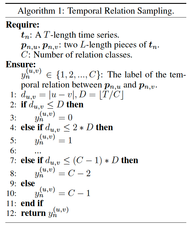
Step 1) sample different types of temporal relation
- step 1-1) sample two \(\boldsymbol{p}_{n, u}\) & \(\boldsymbol{p}_{n, v}\)
- step 1-2) assign temporal relation between \(\boldsymbol{p}_{n, u}\) and \(\boldsymbol{p}_{n, v}\)
- based on temporal distance \(d_{u, v}\) ( where \(d_{u, v}=\mid u-v \mid\) )
step 2) define \(C\) types of temporal relations
-
for each pair of pieces based on their temporal distance
- step 2-1) set a distance threshold as \(D=\lfloor T / C\rfloor\),
- step 2-2) if the distance \(d_{u, v}\) of a piece pair is ….
- \(0 \sim D \rightarrow\) assign relation label as 0
- \(D \sim 2D \rightarrow\) assign relation label as 1
- …
- \(CD \sim (C+1)D \rightarrow\) assign relation label as C
step 3) extract representations of time pieces
- Based on “sampled time pieces” & “their temporal relations”
- use shared backbone encoder \(f_\theta\)
- extracted feature : \(\boldsymbol{z}_{n, u}=f_\theta\left(\boldsymbol{p}_{n, u}\right)\) & \(\boldsymbol{z}_{n, v}=f_\theta\left(\boldsymbol{p}_{n, v}\right)\)
step 4) construct the temporal relation representation
- as \(\left[\boldsymbol{z}_{n, u}, \boldsymbol{z}_{n, v}\right]\).
step 5) relation reasoning
-
input : \(\left[\boldsymbol{z}_{n, u}, \boldsymbol{z}_{n, v}\right]\)
- model : relation reasoning head \(r_{\varphi}(\cdot)\)
- output : final relation score ( = \(h_n^{(u, v)}=r_{\varphi}\left(\left[\boldsymbol{z}_{n, u}, \boldsymbol{z}_{n, v}\right]\right)\) )
- task : multi-class classification problem
- loss function : CE Loss ( \(\mathcal{L}_{\text {intra }}=-\sum_{n=1}^N y_n^{(u, v)} \cdot \log \frac{\exp \left(h_n^{(u, v)}\right)}{\sum_{c=1}^C \exp \left(h_n^{(u, v)}\right)}\) )
(3) Summary
Jointly optimize 2 loss functions : \(\mathcal{L}=\mathcal{L}_{\text {inter }}+\mathcal{L}_{\text {intra }}\)
SelfTime
- efficient algorithm compared with the traditional contrastive learning models such as SimCLR
- complexity
- SimCLR : \(O\left(N^2 K^2\right)\)
- SelfTime : \(O\left(N K^2\right)+O(N K)\)
- \(O\left(N K^2\right)\) : complexity of inter-sample relation reasoning module
- \(O(N K)\) : complexity of intra-tempora relation reasoning module