(paper 56) SS Pre-training for TSC

Self-Supervised Pre-Training For TS Classification

Contents

1. Abstract
2. Preliminaries
3. Approach
   1. Encoder
   2. Self Supervised Pre-training

0. Abstract

Self-supervised TS pre-training

• propose a novel end-to-end neural network architecture based on self-attention

• suitable for …
  • (1) capturing long-term dependencies
  • (2) extracting features from different time series
• propose two different self-supervised pretext tasks for TS
  • (1) Denoising
  • (2) Similarity Discrimination based on DTW

1. Preliminaries

Notation :

• N TS : \(\boldsymbol{X}=\left\{\boldsymbol{x}_1, \boldsymbol{x}_2, \ldots, \boldsymbol{x}_N\right\}\)

• TS by time : \(\boldsymbol{x}=\left\{\left\langle t_1, \boldsymbol{v}_1\right\rangle,\left\langle t_2, \boldsymbol{v}_2\right\rangle, \ldots,\left\langle t_m, \boldsymbol{v}_m\right\rangle\right\}\)

  • \(m\) : length of TS

  • \(\boldsymbol{v}_i \in \mathbb{R}^d\),

  • If interval in TS are same : \(\Delta t=t_{i+1}-t_i\)

    \(\rightarrow\) \(\boldsymbol{x}=\left\{\boldsymbol{v}_1, \boldsymbol{v}_2, \ldots, \boldsymbol{v}_m\right\}\)

• sub series : \(\left\{\boldsymbol{v}_i, \ldots, \boldsymbol{v}_j\right\}\) ( = \(\boldsymbol{x}[i: j]\) )

• labeled TS : \(\boldsymbol{D}=\left\{\left\langle\boldsymbol{x}_1, y_1\right\rangle,\left\langle\boldsymbol{x}_2, y_2\right\rangle, \ldots,\left\langle\boldsymbol{x}_N, y_N\right\rangle\right\}\)

  • \(\boldsymbol{D}_{\text {train }}\) & \(\boldsymbol{D}_{\text {test }}\)

Model : \(\mathcal{F}(\cdot, \boldsymbol{\theta})\)

• part 1) \(\mathcal{F}\left(\cdot, \boldsymbol{\theta}_{\text {backbone }}\right)\)
• part 2) \(\mathcal{F}\left(\cdot, \theta_{c l s}\right)\)

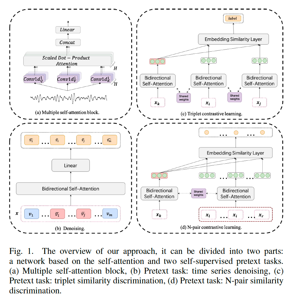
2. Approach

divided into 2 parts:

• (1) a network based on the self-attention
  • introduce Encoder
• (2) two self-supervised pretext tasks

(1) Encoder

based on self-attention

Advantages :

• (1) captures longer dependence than RNN or TCN
• (2) ( \(\leftrightarrow\) RNN ) can be trained in parallel & more efficient
• (3) can handle variable-length time series like RNN and TCN

self-attention block generally consists of 2 sub-layers

• (1) multi-head self-attention layer
  • \(\operatorname{MultiHead}\left(\boldsymbol{x}^l\right)=\operatorname{Concat}\left(\operatorname{head}_1, \ldots, \text { head }_H\right) \boldsymbol{W}^O\).
    • head \(_i=\) Attention \(\left(\operatorname{Conv} 1 \mathrm{~d}_i^Q\left(\boldsymbol{x}^l\right),\operatorname{Conv}^2 \mathrm{~d}_i^K\left(\boldsymbol{x}^l\right), \operatorname{Conv} 1 \mathrm{~d}_i^V\left(\boldsymbol{x}^l\right)\right)\)
    • \(W^O \in \mathbb{R}^{d \times d}\).
• (2) feed-forward network

Differences from Transformer

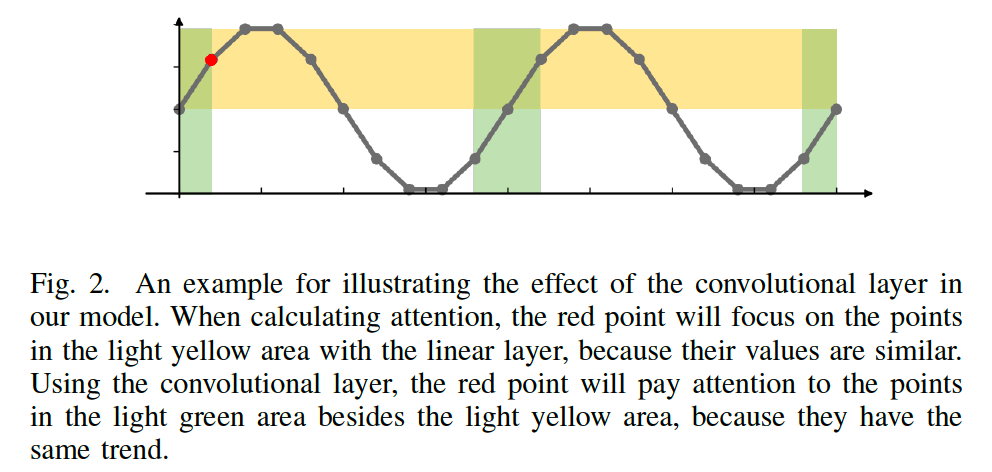
• (1) the original linear layer is replaced by a series of convolution layers

  • ( time series should be tokenized first )
  • CNN with different kernel sizes
  • linear layer : only capture features simultaneously
  • convolutional layer : capture features in a period

  

• (2) TS data «< NLP data

  • be caution of overfitting! Not to much parameters

• (3) TS are longer than the series in NLP

  • only calculate part of the attention to solve this problem

  • partial attention : includes …

    • local attention at all positions

    • global attention at some positions.

(2) Self Supervised Pre-training

features in TS :

• (1) local dependent features
• (2) overall profile features

introduce SSL task for TS

• (1) Denoising
• (2) Similarity Discrimination based on DTW

a) Denoising

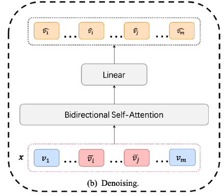
• Task : TS denoising & reconstruction

• Goal : capture the local dependence and change trend.

• Procedures :

  • Add noise to entire sub-sequence during training
    • (NLP) one word = (TS) one sub-sequence
    • thus, add to ENTIRE sub-sequence
  • Make model remove the noise
    • based on 2-way context information

Notation

• (before noise) \(\boldsymbol{x}=\left\{\boldsymbol{v}_1, \boldsymbol{v}_2, \ldots, \boldsymbol{v}_m\right\}\)
  • add noise to \(\boldsymbol{x}[i: j]\)
• (after noise) \(\left\{\boldsymbol{v}_1, \ldots, \overline{\boldsymbol{v}}_i, \ldots, \overline{\boldsymbol{v}}_j, \ldots, \boldsymbol{v}_m\right\}\)
  • \(\overline{\boldsymbol{v}}_k=\boldsymbol{v}_k+\boldsymbol{d}_{k-i}(1 \leq k \leq m)\),
• (model) \(\mathcal{F}_{\boldsymbol{D}}(\cdot)\)
• (model output) \(\mathcal{F}_{\boldsymbol{D}}(\overline{\boldsymbol{x}})=\left\{\hat{\boldsymbol{v}}_1, \ldots, \hat{\boldsymbol{v}}_m\right\}\)

Loss function (MSE) :

• \(L_{\text {Denoising }}=\sum_{k=1}^m\left(\boldsymbol{v}_k-\hat{\boldsymbol{v}}_k\right)^2\).

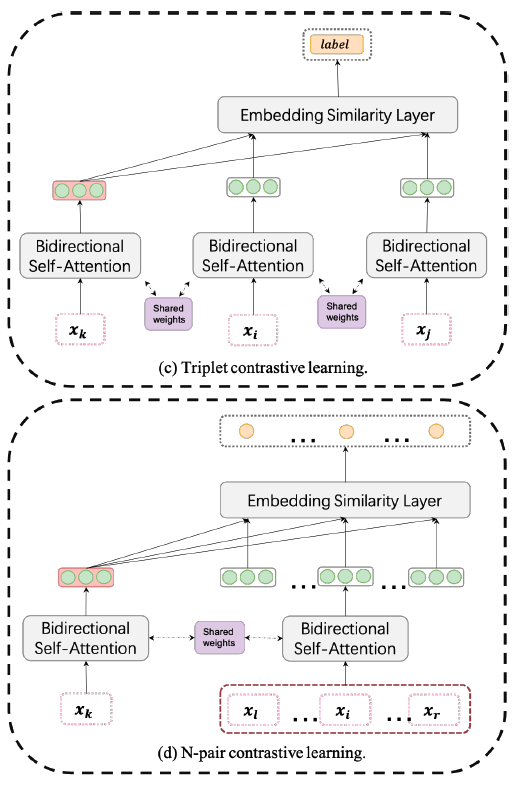
b) Similarity Discrimination based on DTW

• Goal : focus on the TS global features

• How : measure the similarity of TS through DTW ( instead of real labels )

• Procedures :

  • randomly select 3 samples \(\boldsymbol{x}_k, \boldsymbol{x}_i\) and \(\boldsymbol{x}_j\)

    • anchor (1) : \(\boldsymbol{x}_k\)
    • others (2) : \(\boldsymbol{x}_i, \boldsymbol{x}_j\)

  • Binary Classification ( BCE loss )

    • model judges whether \(\boldsymbol{x}_k\) is more similar to \(\boldsymbol{x}_j\) than \(\boldsymbol{x}_i\)
    • \(\text { label }= \begin{cases}1, & \mathrm{DTW}\left(\boldsymbol{x}_k, \boldsymbol{x}_j\right) \geq \operatorname{DTW}\left(\boldsymbol{x}_k, \boldsymbol{x}_i\right) \\ 0, & \text { otherwise }\end{cases}\).

    \(\rightarrow\) triplet similarity discrimination ( Fig 1(c) )

• extend to N-pair contrastive learning

  • for \(\boldsymbol{x}_k\), the model needs to select the \(\beta\) most similar samples from \(n\) samples
  • Binary CLS \(\rightarrow\) \(n\) multi-label CLS ( CE loss )

Notation

• loss function : \(L_{D T W}\)
• set \(\Phi\) : consistsof the id of the \(\beta\) most similar samples
• set \(\Psi=\{1, \ldots, n\}\) : id of all samples
• output of model : \(\mathcal{F}_{\boldsymbol{S}}\left(\boldsymbol{x}_k, \boldsymbol{x}_1, \ldots, \boldsymbol{x}_n\right)\)

Loss function :

• \(\begin{aligned} L_{D T W}=-& \sum_{i \in \Phi} \log \left(\mathcal{F}_{\boldsymbol{S}}\left(\boldsymbol{x}_k, \boldsymbol{x}_1, \ldots, \boldsymbol{x}_n\right)[i]\right)- \sum_{i \in(\Psi-\Phi)} \log \left(1-\mathcal{F}_{\boldsymbol{S}}\left(\boldsymbol{x}_k, \boldsymbol{x}_1, \ldots, \boldsymbol{x}_n\right)[i]\right) \end{aligned}\).

3. Experiment

(1) Dataset

Classification Task

UCR Time Series Classification Archive 2015, 85 datasets

• each dataset : TRAIN & TEST ( ratio not fixed )
• 65 datasets : TEST > TRAIN
  • # of class : (min) 2 & (max) 60
  • seq length : (min) 24 & (max) 2709

Prediction Task

real data from website : power demand ( of Dutch research )

• length : 35040
  • (max) 2152
  • (min) 614

(2) Experiment Settings

use \(H=12\) Self-attention block convolution kernel size :

• {3, 5, 7, 9, 11, 13, 15 ,17, 19, 21, 23, 25}

Backbone = Stack 4 multiple self-attention blocks

Add 1~2 conv layers on the backbone for specific tasks

Loss function :

• CLS : CE loss
• REG : MSE loss

(3) Ablation Study

2 aspects

• (1) effectiveness of conv layer
• (2) way of adding noise ( in pretext A )

use CLS task to quantify the performance

a) Effectiveness of conv layer

in Self-attention…

• option 1) FC layer
• option 2) Conv layer

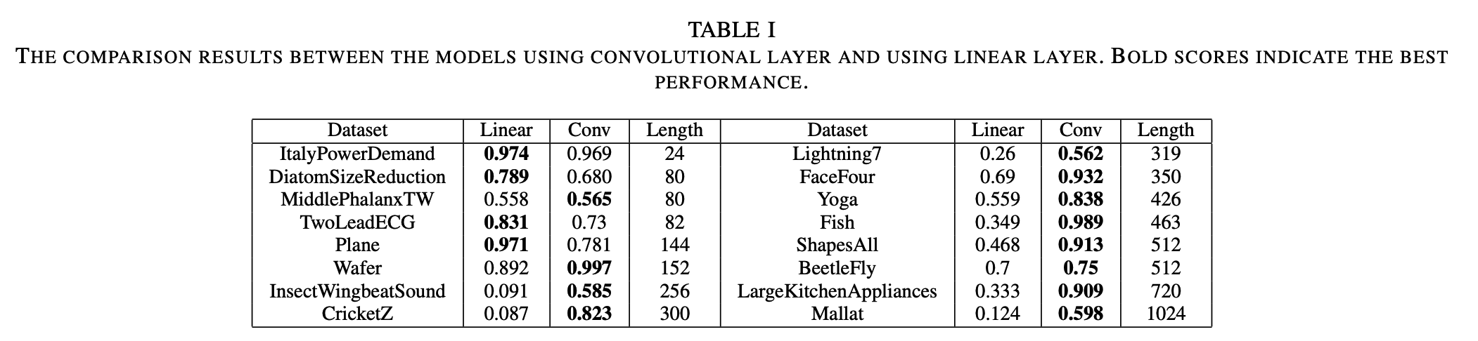
TS length :

• (1) short : linear \(\approx\) conv
• (2) long : conv > linear

b) Way of adding noise

many ways to add noise

compare two ways : adding noise to…

• (1) the sub-series of the TS
• (2) several moments in the TS

(1) the sub-series of the TS

• randomly select a sub-series, whose length is 70% of the original TS
• add Gaussian white noise

(2) several moments in the TS

• add Gaussian white noise at the randomly selected 70% \(\times\) TS length moments
• compare the differences, by visualizing the features obtained by the trained model
  • use t-SNE for dim-reduction & visualize

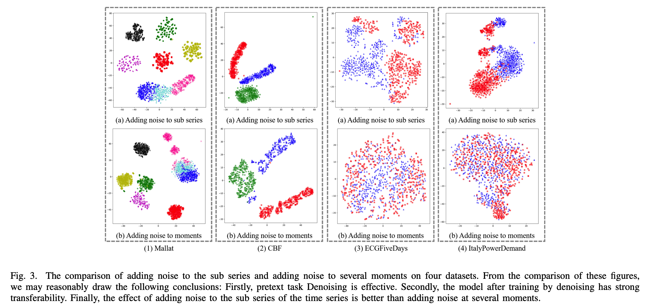
Fig.3(1)(a)

• denoising pre-training is effective!
• \(\because\) easy to determine the classes through the features extracted by the model

Fig.3(1,2,3,4)(a)

• after training by denoising, has strong transferability

\(\rightarrow\) effect of adding noise to the sub-series > adding noise at several moments