(paper 57) Contrastive Learning based self-supervised TS analysis

Contrastive Learning based self-supervised TS

Contents

1. Abstract
2. Introduction
3. Related Work
   1. Contrastive Learning
   2. DA for TS data
4. Self-Supervised TS Analysis
   1. Problem Statement
   2. SimCLR
   3. SimCLR-TS
   4. CNN-1D encoder
   5. Data Augmentation

0. Abstract

SSL : usually accomplished with some sort of data augmentation

This paper :

• presents a novel approach for SSL based TS anlaysis, based on SimCLR
• present novel data augmentation
  • focusing especially on TS data

1. Introduction

propose SimCLR-TS

• SimCLR ssl based industrial TS analysis framework,
• SimCLR framework
  • composition of multiple data-augmentation techniques

Conventional Data Augmentations

• ex) rotation, crop and resize and color distortion

  \(\rightarrow\) cannot be applied as they are for TS

  ( \(\because\) inherent characteristics of temporal and dynamic dependencies in MTS )

\(\rightarrow\) Propose multiple augmentation techniques for TS

2. Related work

(1) Contrastive learning

proposed contrastive learning methods can be categorized into …

• (1) Context-Instance contrast methods
  • ex) principle of predicting relative position
  • ex) maximizing mutual information
• (2) Context-Context contrast methods
  • learning in a discriminative fashion from individual instances.
  • ex) deep clustering approach
    • Swapping Assignment between multiple Views (SwAV)

Similar works to our proposed :

( both deal with very specific signals )

• (1) CLAR
• (2) SeqCLR

\(\leftrightarrow\) proposed : deal with MTS of a arbitrary and mixed physical units which can affect the choice of suitable augmentations

a) CLAR

• classification of audio samples based on SimCLR

• also utilize time–frequency domain

  ( \(\leftrightarrow\) proposed : work only on the raw data & do not need to deal with multiple channels of different signals )

• pre-training is not fully unsupervised

  \(\rightarrow\) just aimed for boosting the raw performance

  ( \(\leftrightarrow\) proposed : aim to create the most meaningful latent representation in a fully unsupervised way )

• train their evaluation head always on the fully labeled data

  ( \(\leftrightarrow\) train our final classifier with only fractions of the labeled data )

b) SeqCLR

• specifically concerned with EEG signals

• aim to extract features from a single channel & to learn a corresponding representation for this single channel

• \(\therefore\) feed their data sequentially!

  ( \(\leftrightarrow\) feed and process multichannel data of different physical units simultaneously )

• combine channels to form new ones & recombination of different datasets as a significant performance booster

  \(\rightarrow\) not applicable with arbitrary multichannel time-series data

(2) Data-augmentation for TS data

a) NLP

• either replacing a token with its synonym
• generating new data samples with back-translation

\(\rightarrow\) cannot be transferred to the general TS

b) TS

• categorized into

  • (1) time-domain
  • (2) frequency domain
  • (3) hybrid approaches
• this paper focus on … (1) time-domain DA

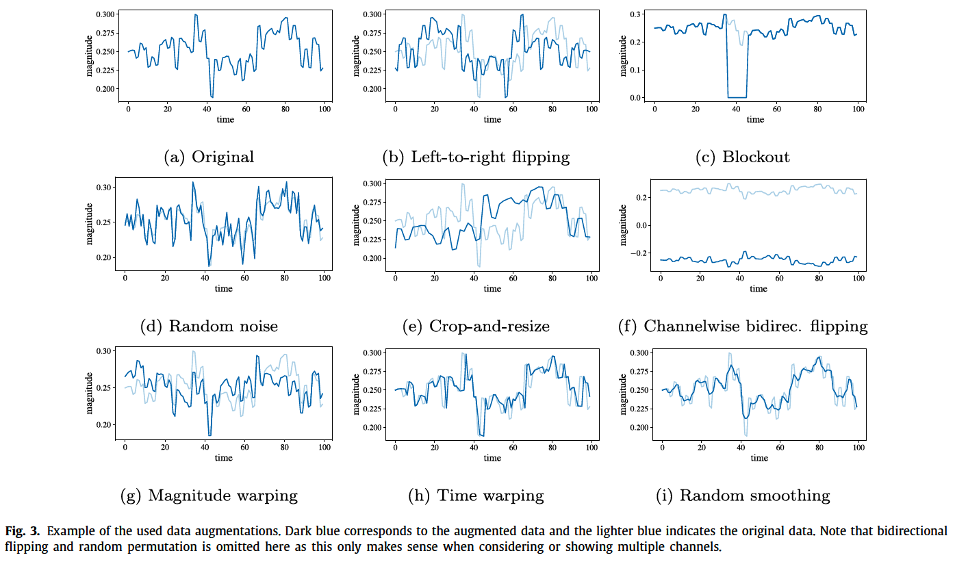
  • ex) window warping

    • speeding up (upsampling) and slowing down (down-sampling) of the time-series

    • larger time-series signal is splitted into multiple smaller signals

      and a moving average smoothing with different window

  • ex) jittering, scaling, rotating, permutating, magnitude warping and time warping
  • ex) Dynamic Time Warping (DTW) Barycentric Averaging (DBA) :
    • weighted version of the time series averaging method
    • propose 3 weighting methods to choose the weights to assign to theseries of the dataset
• this paper aims to to achieve augmentation strategy to have uniform features that preserves maximal information and aligned features for similar examples

3. Self-Supervised TS Analysis

(1) Problem Statement

Assumptions :

1. have a dataset of TS from arbitrary sources
   • these sources can generate either discrete/continuous values

2. No feature extraction techniques have been used

   • input : raw TS

   • only normalization has been used

3. No additional statistical test have been undertaken

Notation

• MTS : \(\left\{\mathbf{x}_1, \mathbf{x}_2, \ldots, \mathbf{x}_T\right\}\) where \(\mathbf{x}_i \in \mathbb{R}^m\),
• \(m\) : number of variables
• \(T\) : length of TS
• labels : \(\left\{y_1, y_2, \ldots, y_T\right\}\)

• neural network : \(f(\cdot)\)

• linear classifier : \(g(\cdot)\)

(2) SimCLR

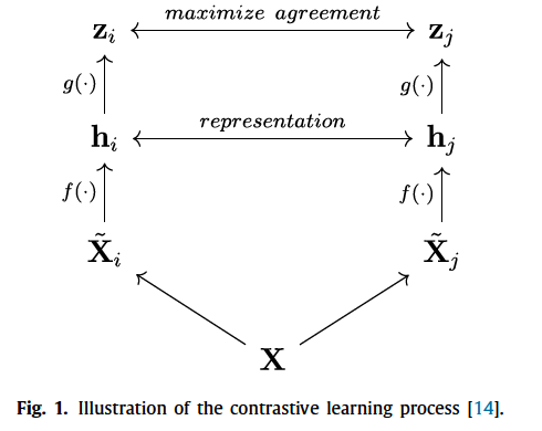
• \(l_{i, j}=-\log \frac{\exp \left(\operatorname{sim}\left(\mathbf{z}_i, \mathbf{z}_j\right) / \tau\right)}{\sum_{k=1}^{2 N} \mathbb{1}_{k \neq i} \exp \left(\operatorname{sim}\left(\mathbf{z}_i, \mathbf{z}_k\right) / \tau\right)}\).

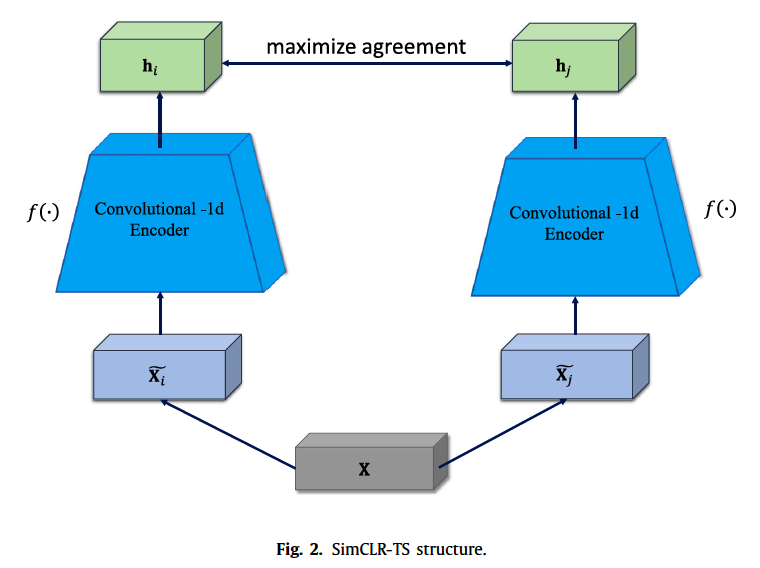
(3) SimCLR-TS

subtle differences

• diff 1 : consider TS instead of images

• diff 2 : \(f(\cdot)\) structure

  • SimCLR : ResNet-50
  • SimCLR-TS : 1D convolution

• diff 3: refrain from using the additional non-linearity \(g(\cdot)\) during contrastive training

  • experienced no benefit by using the additional network
  • avoid unnecessary computation time and memory consumption.

  \(\rightarrow\) directly train to maximize agreement on the latent representations \(h_i\) and \(h_j\)

  • \(l_{i, j}=-\log \frac{\exp \left(\operatorname{sim}\left(\mathbf{h}_i, \mathbf{h}_j\right) / \tau\right)}{\sum_{k=1}^{2 N} \mathbb{1}_{k \neq i} \exp \left(\operatorname{sim}\left(\mathbf{h}_i, \mathbf{h}_k\right) / \tau\right)}\).

• diff 4 : propose a novel set of DA designed for TS

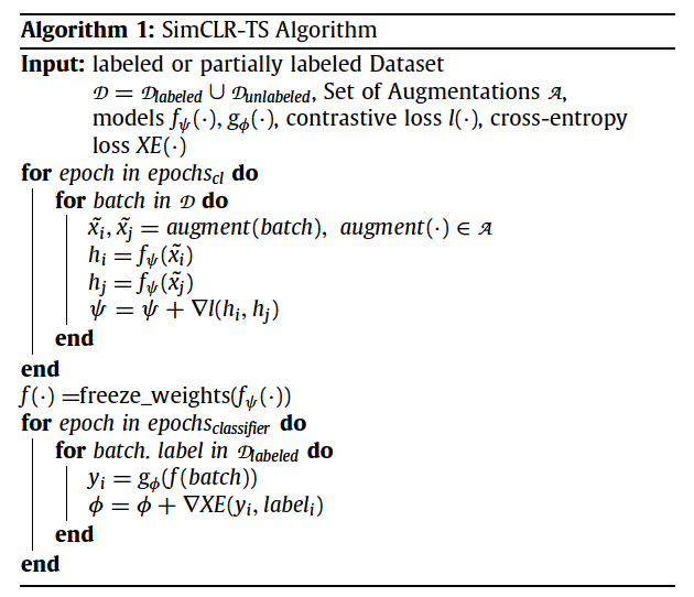
(4) CNN-1D encoder

• receptive field of size \(n_r \times m\)

• strides over \(T \times m\) sequences

• \(p\)-th convolution 1D kernel in the first layer :

  • 2d tensor \(K^{(p)}=\left[k_{i, j}^{(p)}\right] \in \mathbb{R}^{n_r \times m}\)
    • indices \(i, j\) : the dimension along the time and variable

• outputs ( feature maps ) : 1-dim tensor \(H=\left[h_i\right]\).

  • usually use multiple kernels \(\rightarrow\) multiple feature maps

    \(\rightarrow\) 2-dim tensor \(H=\left[h_{i, p}\right]\)

\(\begin{aligned} &h_{i, p}=(x * k)_i=\sum_{g=1}^{n_r} \sum_{f=1}^m x_{i+g-1, f} \cdot k_{g, f}^p \\ &\forall i \in\left\{1, \ldots, T-n_r+1\right\} \\ &\forall p \in\left\{1, \ldots, d_{q+1}\right\}, \end{aligned}\).

• \(h_{i, p}\) : output of the \((i)^{\text {th }}\) receptive field & \(p\)-th kernel
• \(x_{i+g-1, f}\) : elements in the receptive field of the input variable
• \(k_{g, f}\) : kernel
• \(d_{q+1}\) : number of kernels

(5) Data Augmentation