(paper 58) CaSS

CaSS : A Channel-aware Self-supervised Representation Learning Framework for MTS Classification

Contents

1. Abstract
2. Introduction
3. Related Work
   1. Encoder for TSC
   2. Pretext Tasks for TS
4. The framework
5. Channel-aware Transformer (CAT)
   1. Embedding Layer
   2. Co-Transformer Layer
   3. Aggregate Layer
6. Pretext Task
   1. Next Trend Prediction (NTP)
   2. Contextual Similarity (CS)

0. Abstract

Previous works : focus on the pretext task

\(\rightarrow\) neglect the complex problem of MTS encoding

This paper : tackle this challenge from 2 aspects

• (1) encoder
• (2) pretext task

propose a **unified channel-aware self-supervised learning framework CaSS **

• (1) design a new Transformer-based encoder CaT

  ( = Channel-aware Transformer )

• (2) combine 2 novel pretext tasks

  • a) Next Trend Prediction (NTP)
  • b) Contextual Similarity (CS)

1. Introduction

SSL consists of 2 aspects

• (1) encoder
• (2) pretext task

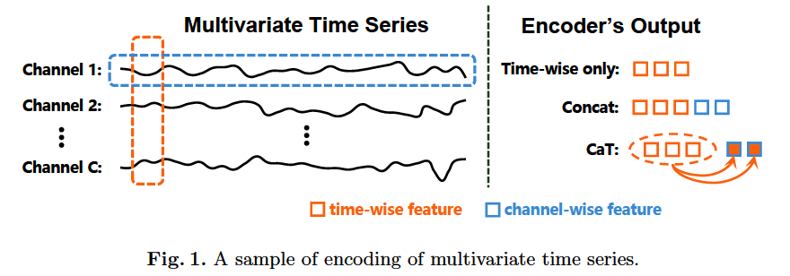
Past works : mostly focus on time-wise features

• where all channel values of one or several time steps are fused through convolution or fully connected layer directly in the embedding process.

\(\rightarrow\) lack of deliberate investigation of the relationships btw channel-wise features

\(\rightarrow\) affects the encoder’s ability to capture the whole characteristics of the MTS

Solutions :

• ex) CNN + RNN

  • RNN : not very suitable for SSL, due to consumption & usually employed in prediction task

• ex) Transformer

  • integrate the features of time-wise and channel-wise

  • becoming more and more popular and is suitable for TS

  • problem : high complexity of computing and space

    \(\rightarrow\) inspires us to design a more effective Transformer-based for MTS

How to integrate “channel-wise features” with pretext task is a challenge

CaSS ( Channel-aware SSL )

(1) Channel-aware Transformer (Cat)

• investigates time-wise and channel-wise features simultaneously

• settings )

  • number of channels of MTS is fixed

    ( usually much less than the time length )

  • time length can be unlimited

• integrate time-wise features into the channel-wise features

  & concatenate all these novel channel-wise features

Design a new self-supervised pretext task

(2-1) Next Trend Prediction (NTP)

• perspective of channel-wise

• in many cases ….

  only the rise & fall of future time ( not exact value ) is necessary

  \(\rightarrow\) cut the MTS from the middle

  & use the previous sequences of all rest channels to predict the trend for each channel

(2-2) Contextual Similarity (CS)

• combines a novel DA strategy to maximize the similarity between similar samples

• learn together with NTP task

  • (1) CS : focuses on the difference between samples
  • (2) NTP : focuses on the sample itself & helps to learn the complex internal characteristics

2. Related Work

(1) Encoder for TSC

Early Works

• combining DTW with SVM
• Time Series Forest
• Bag of Patterns (BOP) & Bag of SFA Symbols (BOSS)
  • dictionary-based classifier. A

\(\rightarrow\) need heavy crafting on data preprocessing & feature engineering

Deep Learning ( CNN based )

• Multi-scale CNN (MCNN)
  • for univariate TSC
• Multi-channel DCNN (MC-DNN)
  • for multivariate TSC
• Hierarchical Attention-based Temporal CNN (HA-TCN) & WaveATTentionNet (WATTNet)
  • apply dilated causal convolution
• Fully Convolutional Network (FCN) &d Residual Network
  • most powerful encoders in multivariate TSC

Deep Learning ( RNN based )

• high computation complexity
• often combined with CNN ( form a two tower structure )

Deep Learning ( Transformer based )

• however … most of them are designed for prediction task

  ( few for TSC )

(2) Pretext Tasks for TS

[15] :

• employs the idea of word2vec

• regards part of the time series as word

  & rest as context

  & part of other time series as negative

[12] :

• employs the idea of contrastive learning

• 2 positive samples are generated by …

  • (1) weak augmentation
  • (2) strong augmentation

  \(\rightarrow\) to predict each other, while the similarity among different augmentations of the same sample is maximized

[13] :

• designed for univariate TS

• samples several segments of the TS

  & labels each segment pairs according to their relative distance in the origin series

• adds the task of judging whether two segments are generated by the same sample

[4] :

• based on sampling pairs of time windows
• predict whether time windows are close in time by setting thresholds

[34] :

• Transformer-based method
• employs the idea of MLM
  • mask operation is performed for MTS
  • encoder is trained by predicting the masked value

Previous works usually focus on time-wise features

& need to continuously obtain the features of several time steps

3. The Framework

focus on SSL for MTS

Notation :

• \(X=\left\{x_0, \ldots, x_M\right\}\) : \(M\) multivariate time series
  • \(x_i \in \mathbb{R}^{C \times T}\) : \(i\)-th TS which has \(C\) channels and \(T\) time steps
• For each \(x_i\) , goal is to generate \(z_i\)

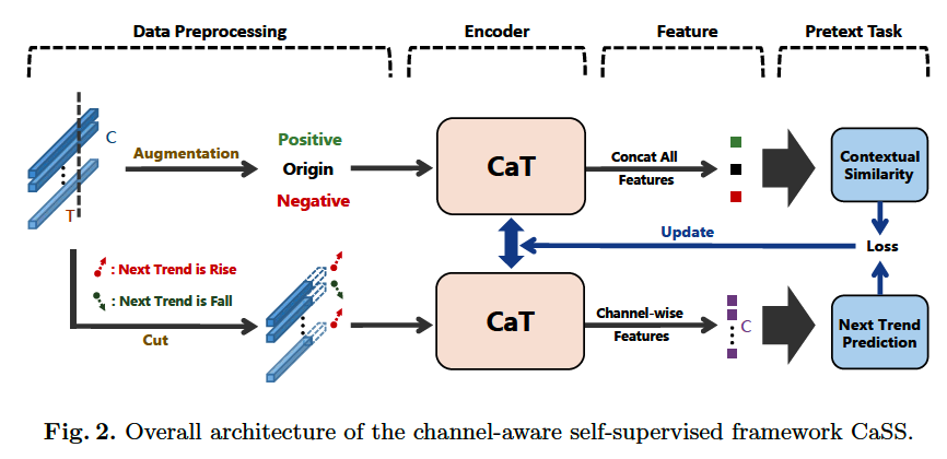
CaSS ( channel-aware self-supervised learning framework )

• (1) proposed novel encoder Channel-aware Transformer (CaT)
• (2) pretext tasks

Channel-aware Transformer (CaT)

• to generate the novel channel-wise features
• generated features are served as the inputs of Next Trend Prediction task and Contextual Similarity task

Procedure

• step 1) preprocess the TS samples

• step 2) apply 2 pretext tasks to learn encoder

• step 3) employ learned representations to other tasks

  ( by freezing the encoder )

4. Channel-aware Transformer (CaT)

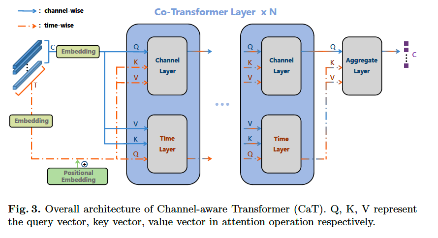
Encoder in SSL framework

Consists of 3 parts

• (1) Embedding Layer
• (2) Co-Transformer Layer : consists of 2 transformer layers
  • a) encode the time-wise features
  • b) encode channel-wise features
  • a) & b) interact with each other
• (3) Aggregate layer
  • fuse the time-wise features into channel-wise features
  • generate final representation

(1) Embedding Layer

[ Input ]

• \(x \in \mathbb{R}^{C \times T}\).

[ Embedding ]

• map it to the \(D\)-dim “time vector space” & “channel vector space”

[ Output ]

• (1) time embedding \(e_t \in\) \(\mathbb{R}^{T \times D}\)
  • \(e_t=x^T W_t+e_{p o s}\).
    • \(W_t \in \mathbb{R}^{C \times D}\) & \(e_{\text {pos }} \in \mathbb{R}^{T \times D}\)
• (2) channel embedding \(e_c \in \mathbb{R}^{C \times D}\)
  • \(e_c=x W_c\).
    • \(W_c \in \mathbb{R}^{T \times D}\).

(2) Co-Transformer Layer

• adopts \(N\)-layer 2 tower structure
  • each layer : composed of “Time layer” & “Channel layer”
  • from \(i\)-th layer ( \(i= 0, \cdots N-1\) ) , obtain the input
    • \(a_t^i \in \mathbb{R}^{T \times D}\) for Time layer
    • \(a_c^i \in \mathbb{R}^{C \times D}\) for Channel layer

Time Layer

( \(a_t^0=e_t, a_c^0=e_c\). )

(1) Query, Key, Value

• \(Q_t^i=a_t^i W_{q t}^i\) ….. input from TIME
• \(K_t^i=a_c^i W_{k t}^i\) ….. input from CHANNEL
• \(V_t^i=a_c^i W_{v t}^i\) ….. input from CHANNEL

(2) Layer Normalization

• \(b_t^i=\operatorname{LayerNorm}\left(\operatorname{MHA}\left(Q_t^i, K_t^i, V_t^i\right)+a_t^i\right)\).
  • MHA : multi-head attention
  • FFN : feed forward network
• \(a_t^{i+1}=\operatorname{LayerNorm}\left(\operatorname{FFN}\left(b_t^i\right)+b_t^i\right)\).

Channel Layer

( \(a_t^0=e_t, a_c^0=e_c\). )

(1) Query, Key, Value

• \(Q_c^i=a_c^i W_{q c}^i\) ….. input from CHANNEL
• \(K_c^i=a_t^i W_{k c}^i\) ….. input from TIME
• \(V_c^i=a_t^i W_{v c}^i\) ….. input from TIME

(2) Layer Normalization

• \(b_c^i=\operatorname{LayerNorm}\left(\operatorname{MHA}\left(Q_c^i, K_c^i, V_c^i\right)+a_c^i\right)\).
  • MHA : multi-head attention
  • FFN : feed forward network
• \(a_c^{i+1}=\operatorname{LayerNorm}\left(\operatorname{FFN}\left(b_c^i\right)+b_c^i\right)\).

(3) Aggregate Layer

Through Co-Transformer Layer…

• obtain time-wise features \(a_t^N\) & channel-wise features \(a_c^N\).

integrate the time-wise features into the channel-wise features

• through attention operation
• ( \(\because\) channel length is usually much less than the time length )

concate these channel-wise features,

as the final representation \(z \in \mathbb{R}^{1 \times(C \cdot D)}\)

(1) Query, Key, Value

• \(Q_c^N=a_c^N W_{q c}^N\).
• \(K_c^N=a_t^N W_{k c}^N\).
• \(V_c^N=a_t^N W_{v c}^N\).

(2) Final Representation

• \(a_c=\operatorname{MHA}\left(Q_c^N, K_c^N, V_c^N\right)\),
• \(z=\left[a_c^1, a_c^2, \ldots, a_c^C\right]\).

5. Pretext Task

design 2 novel pretext tasks

• (1) Next Trend Prediction (NTP)
• (2) Contextual Similarity (CS)

based on our novel channel-wise representation

(1) Next Trend Prediction (NTP)

Input : \(x_i \in \mathbb{R}^{C \times T}\)

Randomly select a time point ( for truncation ) : \(t \in[1, T-1]\)

• part 1 ( before \(t\) step ) : \(x_i^{N T P(t)} \in \mathbb{R}^{C \times t}\)

  • serve as INPUT of NTP task

• part 2 ( after \(t\) step ) : \(y_{i, j}^{N T P(t)}\)

  • \(y_{i, j}^{N T P(t)}=\left\{\begin{array}{ll} 1, \text { if } \quad x_i[j, t+1] \geq x_i[j, t] \\ 0, \text { if } \quad x_i[j, t+1]<x_i[j, t] \end{array},\right.\).

    ( padded with zeros )

    ( \(x_i[j, t]\) : value of \(t\) time step of channel \(j\) in \(x_i\) )

After inputting the NTP sample \(x_i\) into encoder…

\(\rightarrow\) obtain \(z_i^{N T P(t)} \in \mathbb{R}^{C \times D}\)

• where \(z_{i, j}^{N T P(t)} \in \mathbb{R}^D\) : representation of the \(j\)-th channel

Projection head

• applied to predict the probability of “rise” & “fall”

Notation summary

• every sample generated \(K_{NTP}\) input samples

  ( corresponding truncating time point set : \(S \in \mathbb{R}^{K_{N T P}}\) )

• Loss of NTP : \(\ell_{N T P}=\sum_{t \in S} \sum_j^C \operatorname{CE}\left(\varphi_0\left(z_{i, j}^{N T P(t)}\right), y_{i, j}^{N T P(t)}\right)\).

  • \(\varphi_0\) : projection head

(2) Contextual Similarity (CS)

purpose of NTP task

• enable the sample to learn the relationships btw its internal channels

<br.

But also… need to ensure the independence btw different samples

\(\rightarrow\) via Contextual Similarity (CS) task

CS vs Contextual Contrasting task in TS-TCC

• difference : design of the augmentation method
• CS …
  • further applies asynchronous permutation strategy to generate negative samples
  • add the original sample to the self-supervised training

Procedure : generate several positive & negative samples for each sample, through augmentation

(1) Positive samples

• a) Interval Adjustment Strategy

  • randomly selects a series of intervals
  • adjust all values by jittering

• b) Synchronous Permutation Strategy

  • segments the whole TS & disrupts the segment order

  \(\rightarrow\) helps to maintain the relations between segments

(2) Negative samples

• a) Asynchronous Permutation Strategy

  • randomly segments and disrupts the segment order

    ( for each channel in different ways )

batch size \(B\) \(\rightarrow\) \(4B\) augmented samples

( total # of sample in a batch : \(5B\) )

Notation

• input : \(i\)-th sample \(x_i\) in a batch

• representation : \(z_i^0 \in \mathbb{R}^{1 \times(C \cdot D)}\)
• representations of inputs except itself : \(z_i^* \in\) \(\mathbb{R}^{(5 B-1) \times(C \cdot D)}\)
  • where \(z_i^{*, m} \in \mathbb{R}^{1 \times(C \cdot D)}\) is the \(m\)-th representation of \(z_i^*\).
    • 2 positive samples : \(z_i^{+, 1}, z_i^{+, 2} \in \mathbb{R}^{1 \times(C \cdot D)}\)

Loss function : \(\ell_{C S}=-\sum_{n=1}^2 \log \frac{\exp \left(\operatorname{sim}\left(\varphi_1\left(z_i^0\right), \varphi_1\left(z_i^{+, n}\right)\right) / \tau\right)}{\sum_{m=1}^{5 B-1} \exp \left(\operatorname{sim}\left(\varphi_1\left(z_i^0\right), \varphi_1\left(z_i^{*, m}\right)\right) / \tau\right)}\).

• \(\tau\) : hyperparameter
• \(\varphi_1\) : projection head
• sim : cosine similarity

Final SSl loss : combination of NTP & CS loss

• \(\ell=\alpha_1 \cdot \ell_{N T P}+\alpha_2 \cdot \ell_{C S}\).