Semi-Supervised TSC by Temporal Relation Prediction
Contents
- Abstract
- Introduction
- Method
- Training on labeled data
- Training on unlabeled data
0. Abstract
Few efforts consider the underlying temporal relation structure of TS
\(\rightarrow\) propose SemiTime
( = a simple and effective method of Semi-supervised TSC )
For LABELED TS …
- conducts the supervised cls
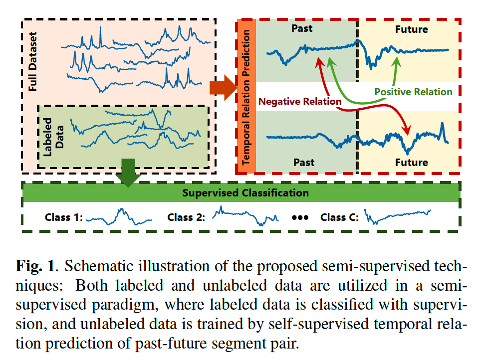
For UNLABELED TS …
-
the segments of past future pair are sampled from TS
-
2 segments of pair from the same TS = positive
( \(\leftrightarrow\) negative )
-
temporal relation between those segments is predicted by SemiTime
By jointly (1) classifying labeled data & (2) predicting the temporal relation of unlabeled data
\(\rightarrow\) useful representation of unlabeled TS can be captured by SemiTime
1. Introduction
underlying temporal relation of TS is a significant supervision signal
propose a general semi-supervised TSC
- by exploring the semantic feature from unlabeled data
2. Method
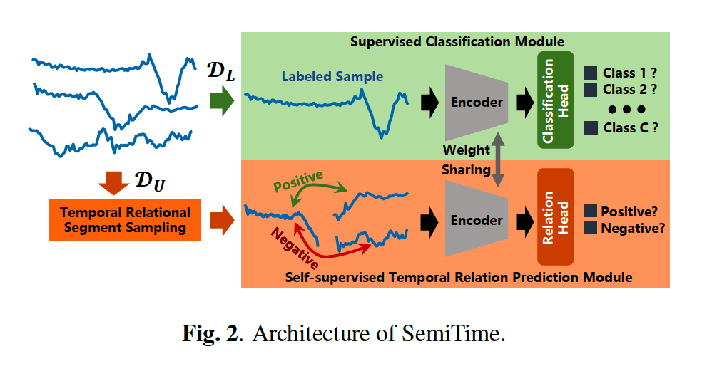
proposed ”SemiTime” consists of 3 modules
- (1) temporal relational segment sampling module
- (2) supervised classification module
- (3) self-supervised temporal relation prediction module
Input : \(\left(\boldsymbol{t}_i, y_i\right) \in \mathcal{D}_L\) & \(\boldsymbol{t}_i \in \mathcal{D}_U\)
- where \(\mathcal{D}_U=\left\{\boldsymbol{t}_i \mid \boldsymbol{t}_i=\left(t_{(i, 1)}, \ldots t_{(i, T)}\right)\right\}_{i=1}^N\) : set of \(T\)-length TS
- where \(\mathcal{D}_L\) is subset of \(\mathcal{D}_U\)
Notation
- backbone encoder : \(f_\theta\)
- classification head : \(h_\mu\)
- relation head : \(h_{\varphi}\)
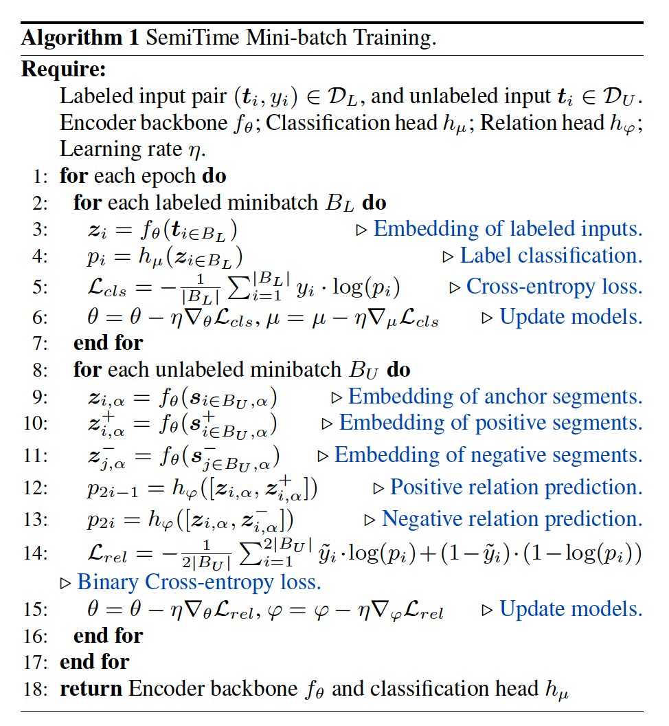
(1) Training on labeled data
Input : \(\left(\boldsymbol{t}_i, y_i\right) \in \mathcal{D}_L\)
Representation : \(\boldsymbol{z}_i=f_\theta\left(\boldsymbol{t}_i\right)\)
CLS output : \(p_i=h_\mu\left(\boldsymbol{z}_i\right)\)
Loss : \(\mathcal{L}_{c l s}=-\frac{1}{ \mid \mathcal{D}_L \mid } \sum_{i=1}^{ \mid \mathcal{D}_L \mid } y_i \cdot \log \left(p_i\right)\).
- CE loss
(2) Training on unlabeled data
Input : \(\boldsymbol{t}_i \in \mathcal{D}_U\)
Split input into two parts
- (1) front \(B\)-length part of \(\boldsymbol{t}_i\) : past segment \(\boldsymbol{s}_{i, \alpha}\)
- (2) rear \((T-B)\)-length part of \(\boldsymbol{t}_i\) : future segment \(\boldsymbol{s}_{i, \alpha}^{+}\)
- where \(B=\lfloor\alpha * T\rfloor\) and \(\alpha\) is a past-future segment split ratio
Anchor & Pos & Neg
- Anchor : \(\boldsymbol{s}_{i, \alpha}\)
- Pos : \(\boldsymbol{s}_{i, \alpha}^{+}\) ( from same TS \(\boldsymbol{t}_i\) )
- Neg : \(s_{j, \alpha}^{-}\)
Representation :
- \(\boldsymbol{z}_{i, \alpha}=f_\theta\left(\boldsymbol{s}_{i, \alpha}\right)\).
- \(\boldsymbol{z}_{i, \alpha}^{+}=f_\theta\left(\boldsymbol{s}_{i, \alpha}^{+}\right)\).
- \(\boldsymbol{z}_{j, \alpha}^{-}=f_\theta\left(s_{i, \alpha}^{-}\right)\).
CLS output :
- \(p_{2 i-1}=h_{\varphi}\left(\left[\boldsymbol{z}_{i, \alpha}, \boldsymbol{z}_{i, \alpha}^{+}\right]\right)\)……… POS relation prediction
- \(p_{2 i}=h_{\varphi}\left(\left[\boldsymbol{z}_{i, \alpha}, \boldsymbol{z}_{i, \alpha}^{-}\right]\right)\)……… NEG relation prediction
Loss : \(\mathcal{L}_{r e l}=-\frac{1}{2 \mid \mathcal{D}_U \mid } \sum_{i=1}^{2 \mid \mathcal{D}_U \mid } \tilde{y}_i \cdot \log \left(p_i\right)+\left(1-\tilde{y}_i\right) \cdot\left(1-\log \left(p_i\right)\right)\)
- binary CE loss
- where \(\tilde{y}_i=1\) denotes positive relation and \(\tilde{y}_i=0\) negative relation