(4) Convex Optimization basics

4. Convex Optimization basics

4-1. Basic Terminology

\(\begin{array}{lr} \operatorname{minimize}_{x \in D} & f(x) \\ \text { subject to } & g_{i}(x) \leq 0, i=1, \ldots, m \\ & h_{j}(x)=0, j=1, \ldots, r, \end{array}\).

• \(f\) & \(g_i\) are all convex
• \(h_j\) are all affine
• optimization domain : \(D=\operatorname{dom}(f) \cap \bigcap_{i=1}^{m} \operatorname{dom}\left(g_{i}\right) \cap \bigcap_{j=1}^{r} \operatorname{dom}\left(h_{j}\right) .\)

Notation

• \(f\) : criterion / objective function
• \(g_i(x)\) : INEQUALITY constraint function

• \(h_j(x)\) : EQUALITY constraint function

• 위 constraint들을 만족하는 점은 feasible point

Optimal values

• 모든 feasible point \(x\) 들 중, \(f(x)\)의 최소값을 optimal value라고 한다

  이 때의 \(x\)는 optimal, solution, minimizer이다

• \(x\)가 feasible하다는 가정 하에,

  • \(f(x) \leq f^{\star}+\epsilon\) 일때의 \(x\)는 \(\epsilon\)-suboptimal

  • \(g_{i}(x)=0\) 일 때, \(g_i\)는 \(x\)에서 active

Convex Minimiaztion = Concave Maximization

\(\begin{array}{lr} \operatorname{maximize}_{x \in D} & -f(x) \\ \text { subject to } & g_{i}(x) \leq 0, i=1, \ldots, m \\ & h_{j}(x)=0, j=1, \ldots, r \end{array}\).

• \(f\) & \(g_i\) are all convex
• \(h_j\) are all affine
• optimization domain : \(D=\operatorname{dom}(f) \cap \bigcap_{i=1}^{m} \operatorname{dom}\left(g_{i}\right) \cap \bigcap_{j=1}^{r} \operatorname{dom}\left(h_{j}\right) .\)

4-2. Convex Solution Sets

\(X_{opt}\) : convex problem 의 Solution Sets

\(\begin{array}{rr} X_{\text {opt }}=\operatorname{argmin}_{x} & f(x) \\ \text { subject to } & g_{i}(x) \leq 0, i=1, \ldots, m \\ & h_{j}(x)=0, i=1, \ldots, r \end{array}\).

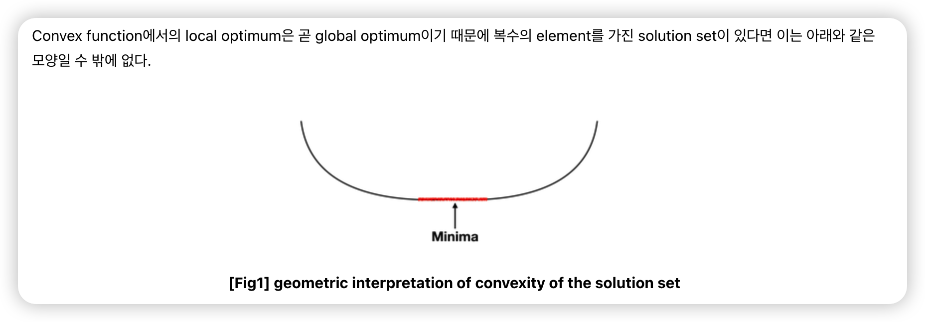
\(X_{opt}\)의 특징

• (1) CONVEX set이다
• (2) \(f\)가 STRICTLY convex하면 UNIQUE한 SOLUTION을 가진다

4-3. First order optimality condition

Convex Problem

• \(\min _{x} f(x) \quad \text { subject to } x \in C\),

First order optimality condition

= (1) iff (2)

• (1) \(\nabla f(x)^{T}(y-x) \geq 0\) for all \(y \in C\)
• (2) 미분가능한 \(f\)에 대해 \(x\)는 optimal solution이다

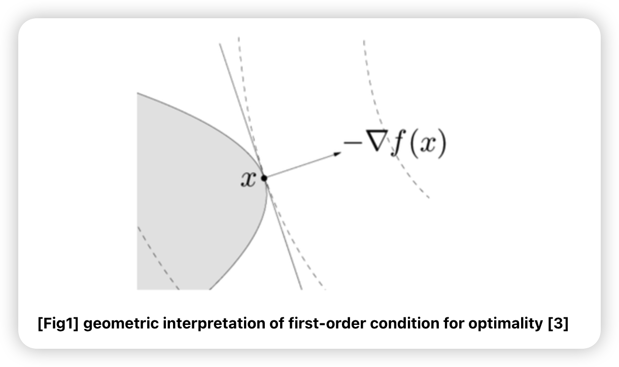
Geometric Interpretation

1. \(\nabla f(x)^{T}(y-x)=0\)는 set \(C\)의 접점 \(x\)를 지나는 hyperplane
   • 아래 그림의 회색 직선
2. \(-\nabla f(x)\) 는 \(x\)에서 optimal point로 향하는 방향이다
3. 위의 (1) 부등식을 만족한다는 것은, set \(C\)가 \(-\nabla f(x)\)의 반대 방향의 half-space를 포함한다는 것이다
   • 회색 직선 왼쪽의 half-space

\(\rightarrow\) 이는 곧 \(x\)가 optimal point임을 의미한다.

Optimality condition : \(\nabla f(x)=0\)

( unconstrained optimization 하에서 )

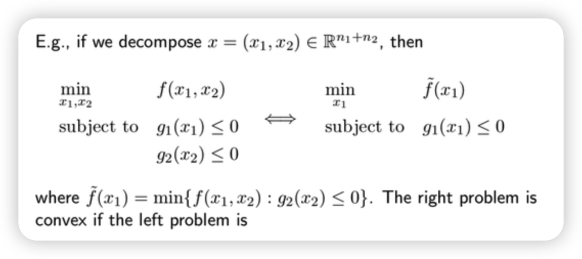
4-4. Partial Optimization

변수 2개 & 제약식 2개의 문제

\(\rightarrow\) 변수 1개 & 제약식 1개 & 변형된 목적함수

Example) hinge form of SVM

SVM의 optimization problem

• \(\min _{\beta, \beta_{0}, \xi} \quad \frac{1}{2} \mid \mid \beta \mid \mid _{2}^{2}+C \sum_{i=1}^{n} \xi_{i}\),
• subject to \(\quad \xi_{i} \geq 0, y_{i}\left(x_{i}^{T} \beta+\beta_{0}\right) \geq 1-\xi_{i}, i=1, \ldots, n\)

[1] 두 개의 제약식을 하나로 합치면…

• subject to \(\xi_{i} \geq \max \left\{0,1-y_{i}\left(x_{i}^{T} \beta+\beta_{0}\right)\right\}\)

[2] 목적함수를 바꿔쓰면…

\(\begin{aligned} \frac{1}{2} \mid \mid \beta \mid \mid _{2}^{2}+C \sum_{i=1}^{n} \xi_{i} & \geq \frac{1}{2} \mid \mid \beta \mid \mid _{2}^{2}+C \sum_{i=1}^{n} \max \left\{0,1-y_{i}\left(x_{i}^{T} \beta+\beta_{0}\right)\right\} \\ &=\min \left\{\frac{1}{2} \mid \mid \beta \mid \mid _{2}^{2}+C \sum_{i=1}^{n} \xi_{i} \quad \xi_{i} \geq 0, y_{i}\left(x_{i}^{T} \beta+\beta_{0}\right) \geq 1-\xi_{i}, i=1, \ldots, n\right\} \\ &=\tilde{f}\left(\beta, \beta_{0}\right) \end{aligned}\).

[3] 정리 ( to UNconstrained problem )

• \(\min _{\beta, \beta_{0}} \frac{1}{2} \mid \mid \beta \mid \mid _{2}^{2}+C \sum_{i=1}^{n} \max \left\{0,1-y_{i}\left(x_{i}^{T} \beta+\beta_{0}\right)\right\}\).

4-5. Transformations & Change of Variables

Theorem 1

\(h: \mathbb{R} \rightarrow \mathbb{R}\) 가 monotone increasing transformation이라면…

\(\begin{array}{cl} \min _{x} f(x) & \text { subject to } x \in C \\ \Longleftrightarrow \min _{x} h(f(x)) & \text { subject to } x \in C \end{array}\).

Theorem 2

\(\phi: \mathbb{R}^{n} \rightarrow \mathbb{R}^{m}\)가 일대일 대응 함수이고, \(\phi\) 의 상(image)이 feasible set \(C\) 를 커버한다면…

\(\begin{array}{cl} \min _{x} f(x) & \text { subject to } x \in C \\ \Longleftrightarrow \min _{y} f(\phi(y)) & \text { subject to } \phi(y) \in C \end{array}\).

4-6. Eliminating equality constraints

Equality Constraints 소거하기

( before )

• \(\min _{x} \quad f(x)\).

• subject to \(\quad g_{i}(x) \leq 0, i=1, \ldots, m\)

  & \(A x=b\)

\(Ax=b\) 를 만족하는 솔루션 \(x_0\)가 있다고 해보자.

\(col(M) = null(A)\) 라면, \(Ax=b\)를 만족하는 임의의 \(x\)를 다음과 같이 표현할 수 있다.

• \(x = My + x_0\).

다시 정리하면,

• \(Ax=A(My+x_0)=AMy + Ax_0 = 0 + b = b\).

자동으로 만족하므로, \(x\)를 위와 같이 치환하여 사용할 경우, 위 제약식을 무시할 수 있다.

( after )

• \(\min _{y} f\left(M y+x_{0}\right)\).
• subject to \(g_{i}\left(M y+x_{0}\right) \leq 0, i=1, \ldots, m\)

유의점

• \(M\)을 계산하는 비용이 큼
• \(x\)가 \(y\)보다 sparse하다면, 더 계산 비용이 커질 수도!

4-7. Slack variables

slack variable \(s\) 를 도입함으로써, 아래의 문제를 다음과 같이 치환하여 풀 수 있다.

• (before) inequality constraint
• (after) equality constraint

( before )

• \(\min _{x} f(x)\),
• \(\begin{array}{r} \text { subject to } \quad g_{i}(x) \leq 0, i=1, \ldots, m \\ A x=b . \end{array}\).

( after )

• \(\min _{x} f(x)\),
• \(\begin{array}{rr} \text { subject to } & s_{i} \geq 0, i=1, \ldots, m \\ &g_{i}(x)+s_{i}=0, i=1, \ldots m \\ & A x=b . \end{array}\).

( 단, \(g_i\)가 affine transform이라 convex problem 이 유지된다 )

4-8. Relaxation

domain set을 넓힌다 ( = 제약을 완화한다 )

( before )

• \(\min _{x} f(x) \text { subject to } x \in C\).

( after )

• \(\min _{x} f(x) \text { subject to } x \in \tilde{C}\).

  where \(\tilde{C} \supseteq C\)

단, 후자를 통해 구해진 optimal value는, 전자를 통해서 구해진 것 보다 더 작거나 같다