(06) Gradient Descent

06. Gradient Descent

6-1. Gradient Descent 란

\(\min _{x} f(x), f:\) differentiable with \(\operatorname{dom}(f)=R^{n}\)

특징

• convex & differentiable \(f\)

• 제약조건 X

Notation

• optimal value : \(f^{*}=\min _{x} f(x)\)
• optimal : \(x^{*}\)

Process ( 표현 1 )

Step 1. 초기 점 \(x^{(0)} \in R^{n}\) 을 선택

Step 2. 아래를 반복

• \(x^{(k)}=x^{(k-1)}-t_{k} \nabla f\left(x^{(k-1)}\right), k=1,2,3, \ldots, t_{k}>0\).
  • \(t_k\) : learning rate / step size ..

Process ( 표현 2 )

Step 1. 초기점 \(\mathrm{x}, x \in \operatorname{dom} f\) 선택

Step 2. 아래를 반복

• (2-1) descent direction \(\Delta x=-\nabla f(x)\) 찾기
• (2-2) Line Search
  • step size \(t>0\) 정하기
• (2-3) \(x=x+t \Delta x\)

Step 3. stopping criterion 충족되면 stop

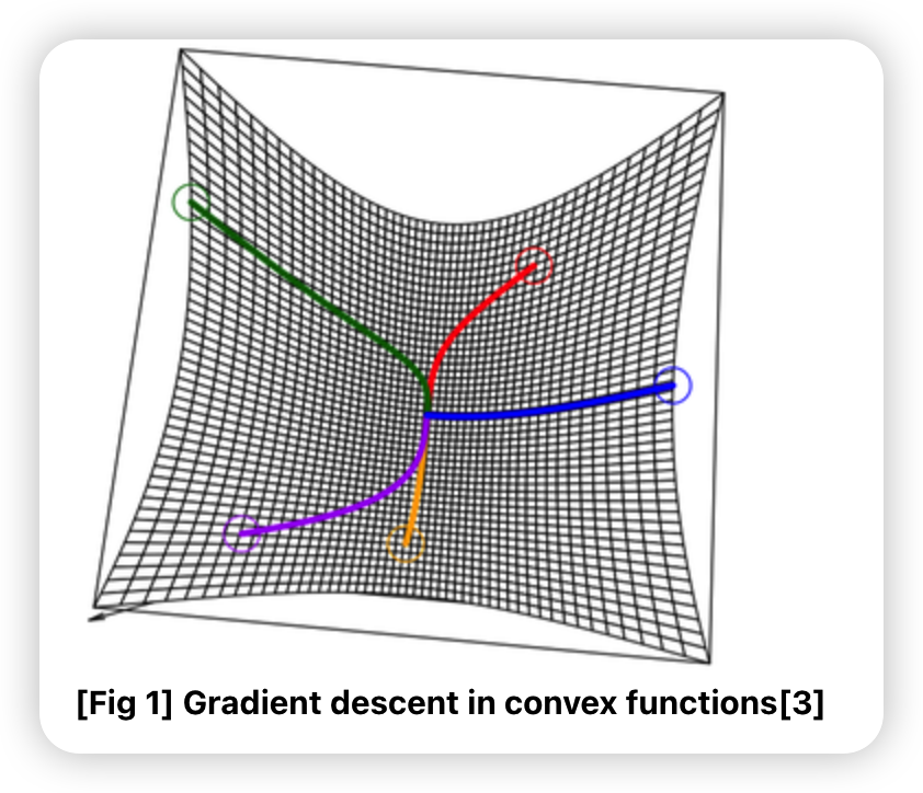
6-2. Gradient Descent in (non-) convex functions

1. convex function
   • local minimum = global minimum
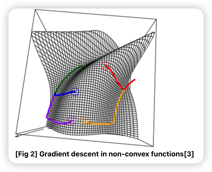
2. non-convex function
   • local minimum = global minimum은 보장 안됨

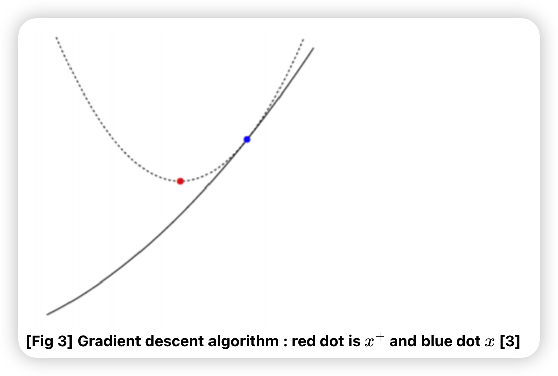
6-3. Gradient Descent Interpretation

Gradient Descent가 담고 있는 의미

• \(f\) 를 2차로 근사한 이후, 함수의 최소 위치를 다음 위치로 선택

Taylor Series Expansion (2차까지)

\(f(y) \approx f(x)+\nabla f(x)^{T}(y-x)+\frac{1}{2} \nabla^{2} f(x)\|y-x\|_{2}^{2}\).

• 위에서, hessian \(\nabla^{2} f(x)\) 를 \(\frac{1}{t} I\) 로 대체하면…

  • \(f(y) \approx f(x)+\nabla f(x)^{T}(y-x)+\frac{1}{2 t}\|y-x\|_{2}^{2}\).

  • hessian을 계산하기엔 computationally expensive..
  • 여기서 \(t\) 는 step size

요약 : ”step size의 역수가 eigen-value인 Hessian”을 2차 항의 계수로 가지는 2차식으로 근사

• 선형 근사 : \(f(x)+\nabla f(x)^{T}(y-x)\)

• proximiity term : \(\frac{1}{2 t}\|y-x\|_{2}^{2}\)

위와 같이 함수를 2차식으로 근사한다.

이 2차식을 최소화 하는 지점을, 다음 지점을 선택한다. ( \(f(y)\)의 gradient가 0이 되는 지점 )

• 다음 지점 : \(y = x^{+}\)

\(\rightarrow\) \(x^{+}=x-t \nabla f(x)\).

6-4. Step Size 고르기

GD를 할 때, step size에 따라 속도 / 발산 issue가 생긴다.

적절한 step size는 어떻게 찾을까?

a) Fixed step size

가장 단순한 방법 ( 어떠한 step에서든 동일한 \(t\) 사용 )

\(t\)가 너무 커도, 너무 작아도 문제다!

example ) \(f(x)=\left(10 x_{1}^{2}+x_{2}^{2}\right) / 2\)

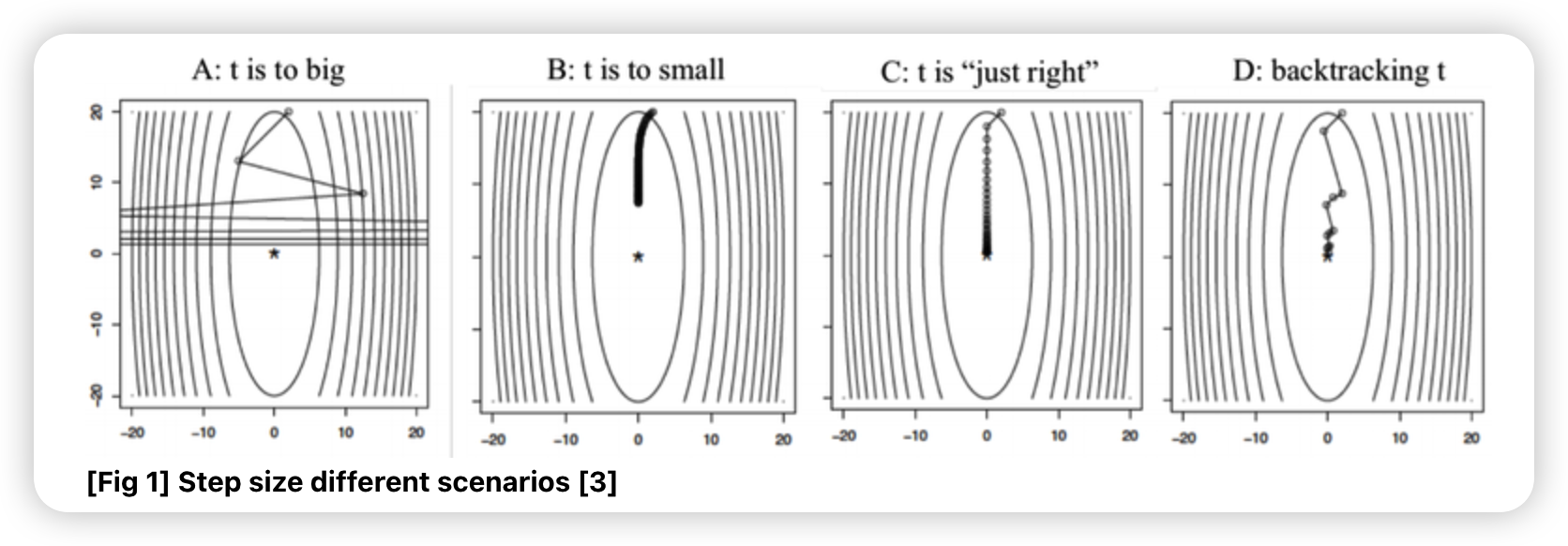
b) Backtracking line search

Fixed step size의 문제점

• 경사가 평평한 구간에서는, optimal point를 지나쳐서 진동할 수도
• 경사가 가파른 구간에서는, 진행이 느릴 수도

\(\rightarrow\) 곡면의 특성에따라 step size를 adaptive하게 조절해야!

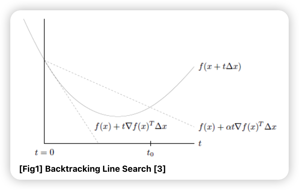
이 중 하나가 backtracking line search

• 아래쪽 점선 : 접선

• 위쪽 점선 : 접선의 기울기에 \(\alpha\)를 곱한 방향으로 한 step을 간 경우

직관적 idea : 한 step을 간 지점에서, \(f(x+t \Delta x)\) 가

• \(f(x)+\alpha t \nabla f(x)^{T} \Delta x\) 위에 있으면 : 너무 큰 step size
• \(f(x)+\alpha t \nabla f(x)^{T} \Delta x\) 아래에 있으면 : 적당한 step size

Process

사용하는 파라미터 : \(\alpha, \beta\)

notation : \(\Delta x=-\nabla f(x)\)

• step 1) initialize \(\alpha, \beta\)
  • \(0<\beta<1\) , \(0< \alpha \leq 1/2\)
• step 2) initialize \(t\)
  • \(t = t_{init} = 1\).
• step 3) 아래를 반복
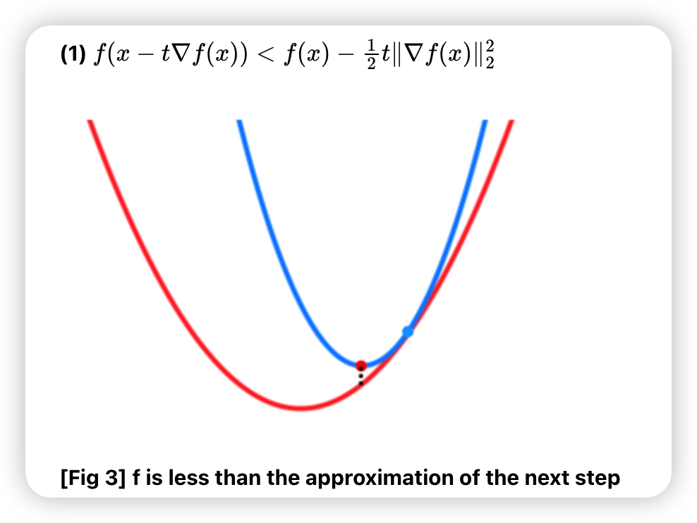
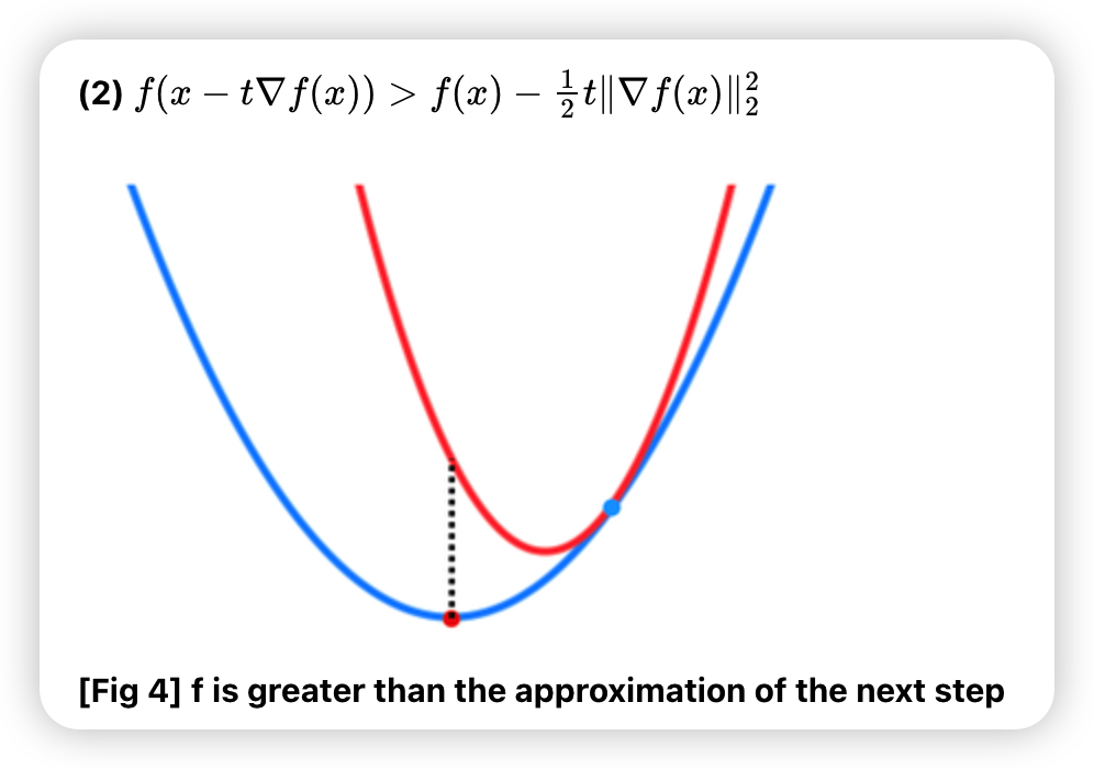
  • \(f(x-t \nabla f(x))>f(x)-\alpha t\|\nabla f(x)\|_{2}^{2}\) 일 경우, \(t=\beta t\) 로 줄이기
  • 위 조건이 만족되지 않을때 까지 반복
• step 4) gradient descent
  • \(x^{+}=x-t \nabla f(x)\).
• stopping criterion을 만족할 때 까지 step 2 ~ step 4 반복

Summary

• simple, but WORKS WELL!
• \(\alpha\) : 다음 step의 방향을 결정
• \(\beta\) : step을 얼마나 되돌아올지 결정
  • \(\beta\) 작을 경우 :
    • 반복은 3번만 하면 됨. ( 조건 금방 충족 )
    • but step size가 작아, 멀ㄹ리 못감
• 대부분 \(\alpha = 1/2, \beta \approx 1\) 로 설정

위의 process의 step3의 조건 :

c) Exact line search

• GD의 곡면의 특성에 맞춰 step size를 adaptive 하게 설정하는 방법 중 하나

• 한 줄 요약 : negative gradient의 직선을 따라, 가장 좋은 step size 설정
• 수식 : \(t=\operatorname{argmin}_{s \geq 0} f(x-s \nabla f(x))\).
• 단점 : 실용적 X
  • step size를 exhaustive하게 탐색

6-3. Convergence Analysis

pass

6-4. Gradient Boosting

https://seunghan96.github.io/ml/ppt/3.Boosting/ 참고

a) Gradient Boosting 이란

• 여러 tree를 ensemble
• GD를 사용하여, 순차적으로 tree 생성
  • 다음 tree : 이전 tree의 오차를 보완하는 방식으로!
• 회귀 & 분류 모두 OK

b) Functional gradient descent

• 함수 공간에 대해서 loss function을 최적화
• gradient의 음수 방향을 가지는 함수를 반복적으로 선택

c) Gradient Boosting ( detail )

Notation

• [x] \(x_i, i=1 \cdots n\)
• [y_true] \(y_i, i=1 \cdots n\)
• [y_pred] \(u_i, i=1 \cdots n\)

Prediction

• weighted average of \(M\) Trees

  ( = \(u_{i}=\sum_{j=1}^{M} \beta_{j} T_{j}\left(x_{i}\right)\) )

Loss Function

• \(\min _{\beta} \sum_{i=1}^{n} L\left(y_{i}, \sum_{j=1}^{M} \beta_{j} T_{j}\left(x_{i}\right)\right)\).

Optimization Problem

• 위의 Loss Function를 최소화하는 \(M\) 개의 가중치 \(\beta_{j}\) 를 찾는 문제
• 재정의 : \(\min _{u} f(u)\)
  • where \(L(y, u)\)

Gradient Boosting :

• 위의 \(\min _{u} f(u)\) 를 gradient descent를 사용해서 풀기

d) Algorithm

• pass

6-5. Stochastic Gradient Descent (SGD)

모든 데이터가 아닌, 하나의 (혹은 소수의) 데이터의 함수값에 대한 gradient만을 구한다.

\(k\) 번째 iteration 에서의 update :

• \(x^{(k)}=x^{(k-1)}-t_{k} \cdot \nabla f_{i_{k}}\left(x^{(k-1)}\right), i_{k} \in\{1,2, \ldots, m\}\).

6-6. Convergence of SGD

GD vs SGD

• GD : batch 방식으로 한번 업데이트 ( = 모든 데이터 사용 )
• SGD : m번의 업데이트 ( = 소수의 데이터만을 사용 )

Updating Equation

• SGD ) \(k\) ~ \(k+m\) step의 업데이트 :
  • \(x^{(k+1)}=x^{(k)}-t_{k} \cdot \sum_{i=1}^{m} \nabla f_{i}\left(x^{(k+i-1)}\right)\).
• GD ) \(k\) ~ \(k+1\) step의 업데이트 :
  • \(x^{(k+m)}=x^{(k)}-t_{k} \cdot \sum_{i=1}^{m} \nabla f_{i}\left(x^{(k)}\right)\).

두 방법 간의 차이 :

• \(\sum_{i=1}^{m}\left[\nabla f_{i}\left(x^{(k+i-1)}\right)-\nabla f_{i}\left(x^{(k)}\right)\right]\).

\(\rightarrow\) 각 \(\nabla f_{i}(x)\) 가 \(x\) 에 대해서 크게 안변한다면 ( = Lipschitz continuous ), SGD도 수렴하게 됨

( if not, 수렴 보장 X )