(paper 84) SSL is More Robust to Dataset Imbalance

SSL is More Robust to Dataset Imbalance

Contents

1. Abstract
2. Introduction
3. Exploring the Effect of Class Imbalance on SSL
   1. Problem Formulation
   2. Experimental Setup
   3. Results
4. Analysis
   1. Rigorous Analysis on a Toy Setting

0. Abstract

Large-scale unlabeled datasets in the wild

\(\rightarrow\) often have LONG-tailed label distributions

This paper : investigate SSL under DATASET IMBALANCE.

Three Findings

Findings 1) off-the-shelf SSL : more ROBUST to class imbalance than SL

• performance gap between balanced & imbalanced pre-training with SSL is smaller than SL

Findings 2) Hypothesize that SSL learns RICHER features from frequent data

• may learn label-irrelevant-but-transferable features that help classify the rare classes and downstream tasks.

  ( \(\leftrightarrow\) SL has no incentive to learn features irrelevant to the labels from frequent examples )

Findings 3) Devise a RE-WEIGHTED REGULARIZATION technique

• that consistently improves the SSL representation quality on imbalanced datasets

1. Introduction

Current SSL algorithms

• mostly trained on curated, balanced datasets

• BUT large-scale unlabeled datasets in the wild

  \(\rightarrow\) imbalanced with a LONG-tailed label distribution

  ( Curating a class-balanced unlabeled dataset requires the knowledge of labels )

Performance of SL degrades significantly on class-imbalanced datasets

Many recent works address this issue with..

• (1) various regularization
• (2) re-weighting/re-sampling techniques

Proposal

Investigate the representation quality of SSL algorithms under class imbalance

\(\rightarrow\) Find out that off-the-shelf SSL are already more robust to dataset imbalance than SL

Evaluate the representation quality by ..

• (1) linear probe on in-domain (ID) data
• (2) finetuning on out-of-domain (OOD) data.

Compare the robustness of SL and SSL representations by “balance-imbalance gap”

= Gap between the performance of the representations pre-trained on

• (1) balanced datasets
• (2) imbalanced datasets

\(\rightarrow\) Gap for SSL is much smaller than SL !!

( This robustness holds even with the same number of samples for SL and SSL, although SSL does not require labels and hence can be more easily applied to larger datasets than SL. )

Why is SSL more ROBUST to dataset imbalance?

• SSL learns richer features from the frequent classes than SL does.
  • help classify the rare classes under ID evaluation
  • transferable to the downstream tasks under OOD evaluation.
• Intuition )
  • Extreme imbalance … important for the models to learn DIVERSE features from the frequent classes which can help classify the RARE classes
  • SL vs SSL
    • SL ) only incentivized to learn those features relevant to predicting frequent classes ( may ignore other features )
    • SSL ) learn the structures within the frequent classes better
      • not supervised or incentivized by any labels

Design a simple algorithm that

• step 1) Roughly estimates the density of examples with KDE
• step 2) Applies a larger sharpness-based regularization

Contributions

• (1) First to systematically investigate the robustness of SSL to dataset imbalance.
• (2) Both empirically and theoretically.
• (3) Principled method to improve SSL under unknown dataset imbalance.

2. Exploring the Effect of Class Imbalance on SSL

How SSL will behave under dataset imbalance

Investigate the effect of class imbalance on SSL

(1) Problem Formulation

a) Class-imbalanced pre-training datasets

Notation

• dimension of input : \(\mathbb{R}^d\)

• number of classes : \(C\)

• \(x\) : input
• \(y\) : label
• Pre-training distn \(\mathcal{P}\) over over \(\mathbb{R}^d \times[C]\)
• \(r\) : ratio of class imbalance
  • \(r=\frac{\min _{j \in[C]} \mathcal{P}(y=j)}{\max _{j \in[C]} \mathcal{P}(y=j)} \leq 1\).

Pre-training distn \(\mathcal{P}\)

• construct distributions with varying imbalance ratios

  ( \(\mathcal{P}^r\) : distribution with ratio \(r\) )

  ( \(\mathcal{P}^{\text {bal }}\) : case where \(r=1\) )

• pre-training dataset \(\widehat{\mathcal{P}}_n^r\) consists of \(n\) i.i.d. samples from \(\mathcal{P}^r\).

Large-scale Data in the wild

• often follow heavily LONG-tailed label distributions ( = \(r\) is small )
• for any class \(j \in[C]\) …
  • (class-conditional distribution) \(\mathcal{P}^r(x \mid y=j)\) is the same across balanced and imbalanced datasets for all \(r\).

b) Pre-trained models

Feature extractor : \(f_\phi: \mathbb{R}^d \rightarrow \mathbb{R}^m\)

• SSL algorithms learn \(\phi\) from unlabeled data.

Linear head : \(g_\theta: \mathbb{R}^m \rightarrow \mathbb{R}^C\)

• Drop the head & only evaluate the quality of feature extractor \(\phi\)

Measure the quality of learned representations on both

• (1) in-domain datasets
• (2) out-of-domain datasets

with either

• (1) linear probe
• (2) fine-tuning

c) In-domain evaluation

Tests the performance of representations

• on the balanced IN-domain distribution \(\mathcal{P}^{\text {bal }}\)
• with linear probe

Settings

• Given \(f_\phi\) ( which is pre-trained on \(\widehat{\mathcal{P}}_n^r\) with \(n\) data points ),

  Train a \(C\)-way linear classifier \(\theta\) on top of \(f_\phi\) on a balanced dataset ( sampled i.i.d. from \(\mathcal{P}^{\text {bal }}\) )

• Metric : Top-1 accuracy

• Results

  • \(A_{\mathrm{ID}}^{\mathrm{SL}}(n, r)\) : ID accuracy of SL representations
  • \(A_{\mathrm{ID}}^{\mathrm{SSL}}(n, r)\) : ~ SSL representations

d) Out-of-domain evaluation

Tests the performance of representations

• by fine-tuning the feature extractor and the head
• on downstream target distribution \(\mathcal{P}_t\).

Settings

• fine-tune \(\phi\) and \(\theta\) ( using the target dataset \(\widehat{\mathcal{P}}_t\) )
• Metric : Top-1 accuracy on \(\mathcal{P}_t\).
• Results : \(A_{\mathrm{OOD}}^{\mathrm{SL}}(n, r)\) & \(A_{\mathrm{OOD}}^{\mathrm{SSL}}(n, r)\)

e) Summary of varying factors

Aim to study the effect of class imbalance to feature qualities on a diverse set of configurations with the following varying factors:

• (1) \(n\) : the number of examples in pre-training
• (2) \(r\) : the imbalance ratio of the pre-training dataset
• (3) ID or OOD evaluation
• (4) SSL algorithms : MoCo v2 & SimSiam

(2) Experimental Setup

a) Dataset

• PRETRAIN on variants of ImageNet or CIFAR-10
  • with a wide range of (1) numbers of examples and (2) ratios of imbalance.
• For LONG-tailed distn …
  • use exponential and Pareto distributions
• Imbalance ratio :
  • \(\{1,0.004,0.0025\}\) for ImageNet
  • \(\{1,0.1,0.01\}\) for CIFAR-10.
• For each imbalance ratio, downsample the dataset with a sampling ratio in \(\{0.75,0.5,0.25,0.125\}\) to form datasets with varying sizes.

ID & OOD evaluation

ID evaluation )

• (1) linear probing : original CIFAR-10 or ImageNet training set
• (2) evaluation : original CIFAR-10 or ImageNet validation set

OOD evaluation )

• case 1) for representations learned on CIFAR-10 :

  • fine tune : with STL-10

• case 2) for representations learned on ImageNet :

  • fine tune : with CUB-200, Stanford Cars, Oxford Pets, and Aircrafts

    ( measure the representation quality with average accuracy on the downstream tasks. )

b) Models

Bacbkones

• (on CIFAR-10) ResNet-18
• (on ImageNet) ResNet-50

Settings :

• Supervised pre-training : standard protocol of He et al. [2016] and Kang et al. [2020].

• Self-supervised pre-training :

  • MoCo v2 & SimSiam

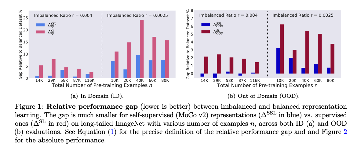
(3) Results : SSL is more robust than SL to Dataset Imbalance

( For both ID & OOD )

• gap of SSL : \(A^{\mathrm{SSL}}(n, 1)-A^{\mathrm{SSL}}(n, r)\)
• gap of SL : \(A^{\mathrm{SL}}(n, 1)-A^{\mathrm{SL}}(n, r)\)

\(\rightarrow\) gap of SSL < gap of SL

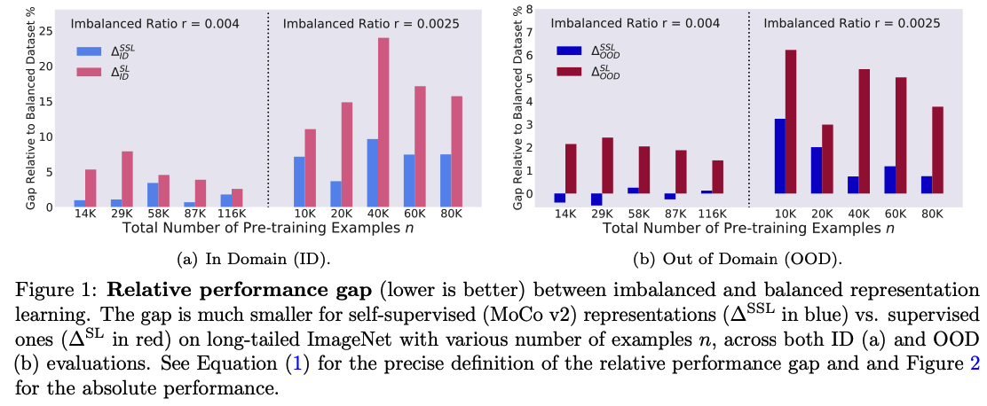
Relative accuracy gap to balanced dataset :

\[\Delta^{\mathrm{SSL}}(n, r) \triangleq\left(A^{\mathrm{SSL}}(n, 1)-A^{\mathrm{SSL}}(n, r)\right) / A^{\mathrm{SSL}}(n, 1)\]

• relative gap of SSL ( between balanced & imbalanced datasets ) : \(\Delta^{\mathrm{SSL}}(n, r)\)
• relative gap of SL ( between balanced & imbalanced datasets ) : \(\Delta^{\mathrm{SL}}(n, r)\)

\(\rightarrow\) relative gap of SSL < relative gap of SL

\(\Delta^{\mathrm{SSL}}(n, r) \triangleq \frac{A^{\mathrm{SSL}}(n, 1)-A^{\mathrm{SSL}}(n, r)}{A^{\mathrm{SSL}}(n, 1)} \ll \Delta^{\mathrm{SL}}(n, r) \triangleq \frac{A^{\mathrm{SL}}(n, 1)-A^{\mathrm{SL}}(n, r)}{A^{\mathrm{SL}}(n, 1)} .\).

Comparing the robustness with the same number of data is actually in favor of SL, because SSL is more easily applied to larger datasets without the need of collecting labels.

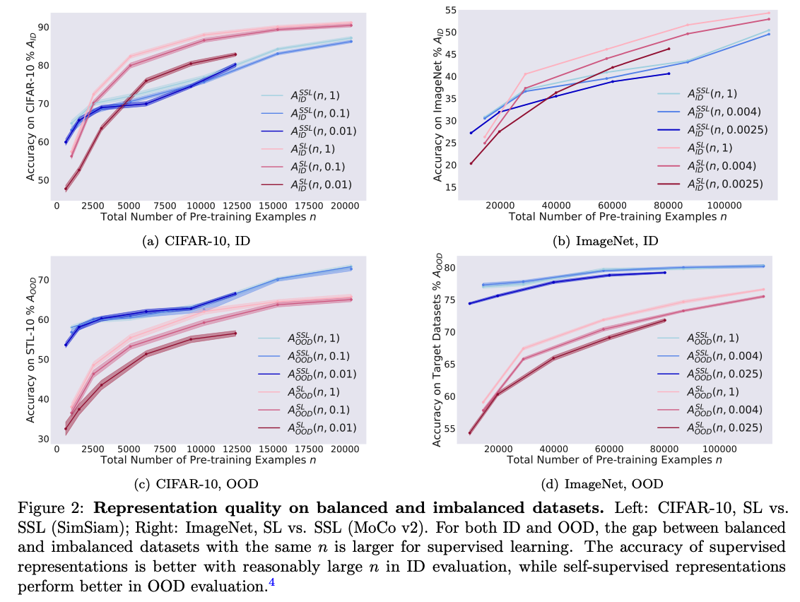
ID vs OOD

representations from SL > SSL … with reasonably large \(n\)

representations from SSL > SL … with OOD settings

• orthogonal to our observation that SSL is more robust to dataset imbalance
• consistent with recent works
  • recent works: SSL performs slightly worse than SL on balanced ID evaluation but better on OOD tasks.

3. Analysis

SSL are more robust to class imbalance than supervised representations.

\(\rightarrow\) Q) Where does the robustness stem from?

SSL learns richer features from frequent data that are transferable to rare data

• Rare classes of the imbalanced dataset : only a few…

  \(\rightarrow\) may want to resort to the features learned from the frequent classes for help.

  \(\rightarrow\) ( but SL … ) learns the features that help classify the frequent classes

  ( + neglect other features which can transfer to the rare classes )

Previous Works

• Meta Learning ( Jamal et al. [2020] ) : explicitly encourage the model to learn features transferable from the frequent to the rare classes

• SSL : learn richer features that capture the intrinsic structures of the inputs

  \(\rightarrow\) useful for classifying the frequent classes and features transferable to the rare classes

(1) Rigorous Analysis on a Toy Setting

SL & SSL setting where the features helpful to classify the frequent classes and features transferable to the rare classes can be clearly separated.

a) Data distribution.

Notation & Settings

• \(e_1, e_2\) : two orthogonal unit-norm vectors in the \(d\)-dim
• pre-training distribution \(\mathcal{P}\)
• 3-way classification problem

Data generation

• Let \(\tau>0\) and \(\rho>0\) be hyperparameters of the distribution

• step 1) Sample \(q\) uniformly from \(\{0,1\}\) and \(\xi \sim \mathcal{N}(0, I)\) from Gaussian distn

• step 2)

  • For the first class \((y=1)\) : set \(x=e_1-q \tau e_2+\rho \xi\).
  • For the second class \((y=2)\) : set \(x=-e_1-q \tau e_2+\rho \xi\).
  • For the third class \((y=3)\): set \(x=e_2+\rho \xi\)

• Classes

  • frequent : class 1 & 2
  • rare : class 3

  ( i.e., \(\frac{\mathcal{P}(y=3)}{\mathcal{P}(y=1)}, \frac{\mathcal{P}(y=3)}{\mathcal{P}(y=2)}=o(1)\). )

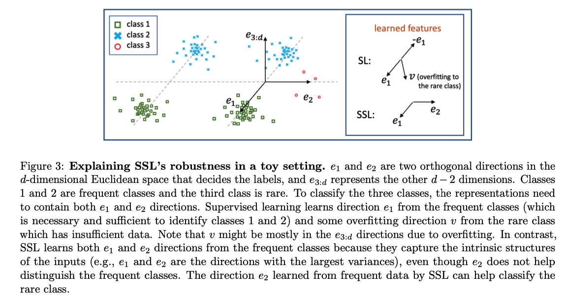
• Both \(e_1\) and \(e_2\) are features from the frequent classes 1 and 2 .
• However, only \(e_1\) helps classify the frequent classes and only \(e_2\) can be transferred to the rare classes.

b) Algorithm Formulations

[ Supervised Learning ]

2-layer NN : \(f_{W_1, W_2}(x) \triangleq\) \(W_2 W_1 x\)

• \(W_1 \in \mathbb{R}^{m \times d}\) and \(W_2 \in \mathbb{R}^{3 \times m}\) for some \(m \geq 3\),
• use \(W_{\mathrm{SL}}=\) \(W_1\) as the feature for downstream tasks.

( Given a linearly separable labeled dataset )

Learn the 2-layer NN with minimal norm \(\mid \mid W_1^{\top} W_1 \mid \mid _F^2+ \mid \mid W_2^{\top} W_2 \mid \mid _F^2\)

• subject to the margin constraint \(f_{W_1, W_2}(x)_y \geq f_{W_1, W_2}(x)_{y^{\prime}}+1\) for all data \((x, y)\) in the dataset and \(y^{\prime} \neq y .^5\)

[ Self-supervised Learning ]

construct positive pairs \(\left(x+\xi, x+\xi^{\prime}\right)\) where \(x\) is from the empirical dataset

• \(\xi\) and \(\xi^{\prime}\) are independent random perturbations.

Learn \(W_{\mathrm{SSL}} \in \mathbb{R}^{m \times d}\) which minimizes \(-\hat{\mathbb{E}}\left[(W(x+\xi))^T\left(W\left(x+\xi^{\prime}\right)\right)\right]+\frac{1}{2} \mid \mid W^{\top} W \mid \mid _F^2\),

• where the expectation \(\hat{\mathbb{E}}\) is over the empirical dataset and the randomness of \(\xi\) and \(\xi^{\prime}\).
• Regularization term \(\frac{1}{2} \mid \mid W^{\top} W \mid \mid _F^2\) : introduced only to make the learned features more mathematically tractable.

c) Main Intuitions

Compare the features learned by SSL and SSL on an imbalanced dataset

• abundant (poly in \(d\) ) number of data from the frequent classes
• small (sublinear in \(d\) ) number of data from the rare class.

Key Intuition :

• SL learns only the \(e_1\) direction (which helps classify class 1 vs. class 2 )

  ( some random direction that overfits to the rare class. )

• SSL learns both \(e_1\) and \(e_2\) directions from the frequent classes.

Results : Since how well the feature helps classify the rare class (in ID evaluation) depends on how much it correlates with the \(e_2\) direction

\(\rightarrow\) SSL provably learns features that help classify the rare class