( 참고 : 패스트 캠퍼스 , 한번에 끝내는 컴퓨터비전 초격차 패키지 )
Representation Learning (1)
1. Metric Learning
(1) Euclidean Distance
- \(D_{E}\left(x_{i}, x_{j}\right)=\sqrt{\left(x_{i}-x_{j}\right)^{\top}\left(x_{i}-x_{j}\right)}\).
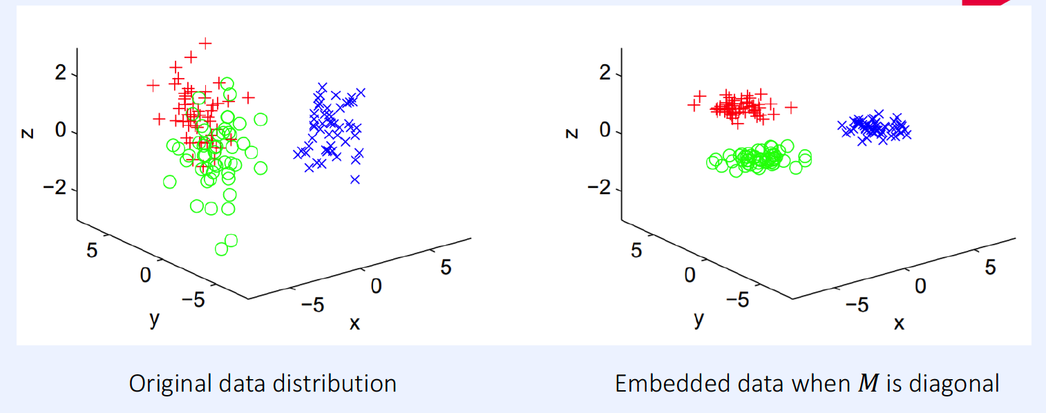
(2) Mahalanobis Distance
- \(D_{M}\left(x_{i}, x_{j}\right)=\sqrt{\left(x_{i}-x_{j}\right)^{\top} M\left(x_{i}-x_{j}\right)}\).
- considering the data manifold!
- Euclidean Distance = special case of Mahalanobis Distance, where \(M=I\)
Mahalanobis Distance in Multivariate Gaussian :
-
\(M = \Sigma^{-1}\).
where \(\mathcal{N}(\mathbf{x})=\frac{1}{\sqrt{(2 \pi)^{k} \mid \Sigma \mid }} \exp \left(-\frac{1}{2}(\mathbf{x}-\boldsymbol{\mu})^{\top} \Sigma^{-1}(\mathbf{x}-\boldsymbol{\mu})\right)\).
Learning Mahalanobis Distance
- estimate \(M\) from data! ( \(M\) : p.s.d )
(3) A first approach to distance metric learning
Notation : 2 sets of data pairs
- \(S^{+}\): The set of similar pairs
- \(S^{-}\): The set of dissimilar pairs
Objective Function
-
\(M^{*}=\underset{M}{\operatorname{argmin}} \sum_{\left(x_{i}, x_{j}\right) \in S^{+}}\left(x_{i}-x_{j}\right)^{\top} M\left(x_{i}-x_{j}\right)\)………… (1)
where \(\text { s.t. } \sum_{\left(x_{i}, x_{j}\right) \in S^{+}}\left(x_{i}-x_{j}\right)^{\top} M\left(x_{i}-x_{j}\right) \geq 1\) ………. (2)
-
Interpretation
- (1) should be small, if similar data
- (2) should be larger than 1, if dissimilar data
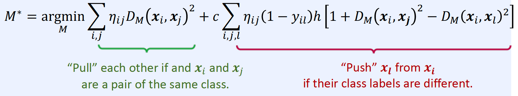
(4) Large Margin Nearest Neighbor (LMNN)
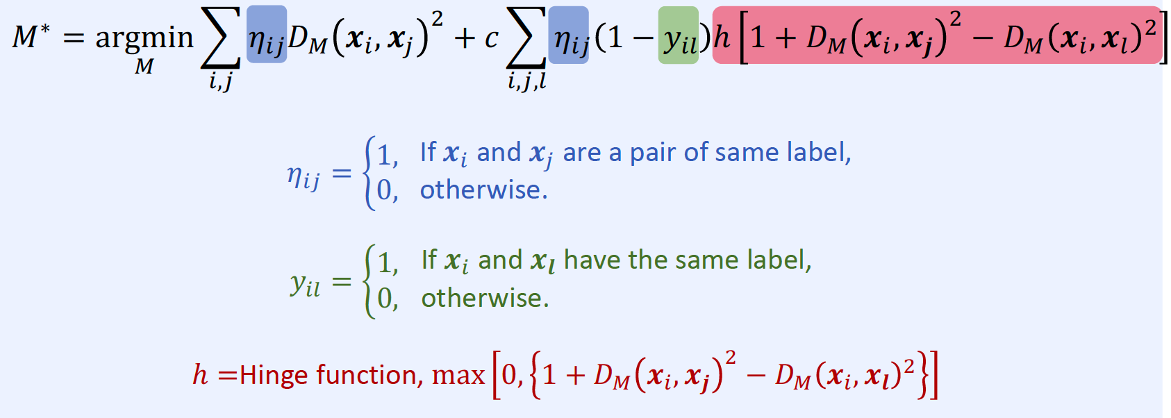
Interpretation
2. Deep Metric Learning
“Learning representation from data”
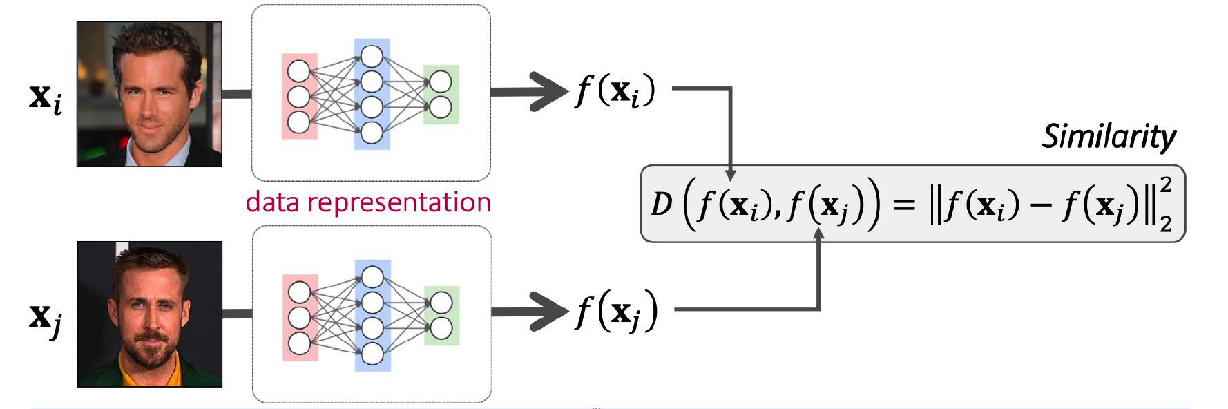
(1) Deep Metric Learning
\(D(f(x_i), f(x_j))\) ,
\(\rightarrow\) Learn function \(f\) that maps data to data representation with DNNs!
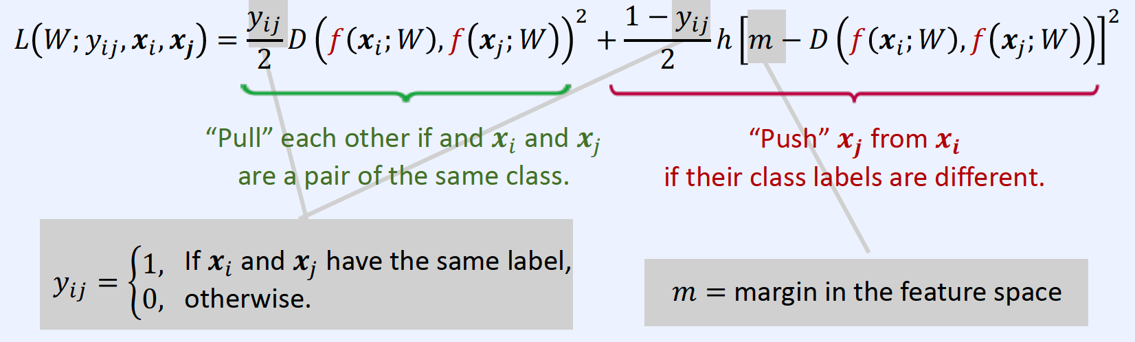
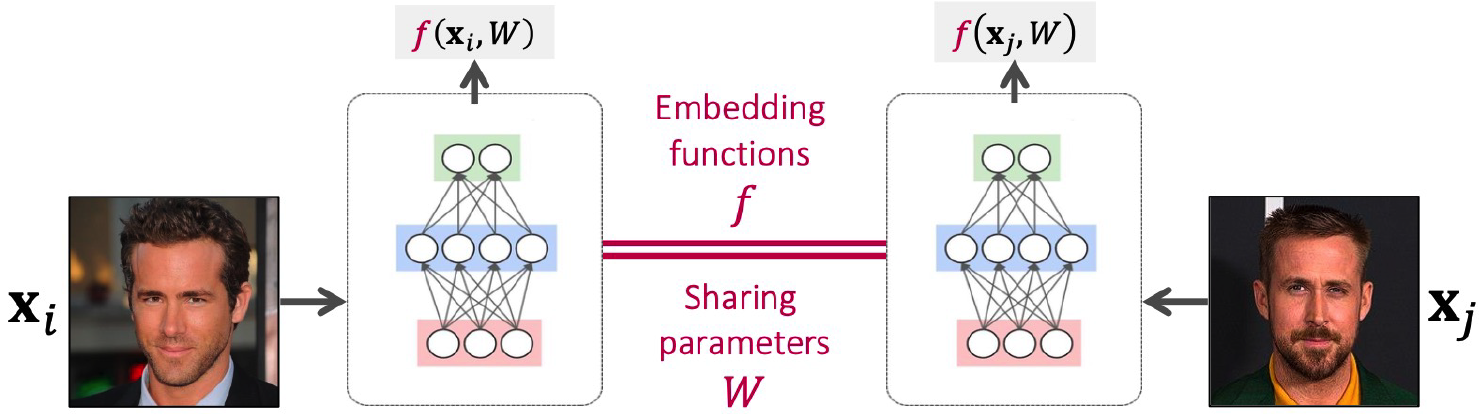
(2) Siamese Network
Siamese = pair of NN, sharing parameters
Contrastive Loss
- make similar pairs close
- make dissimilar pairs far away
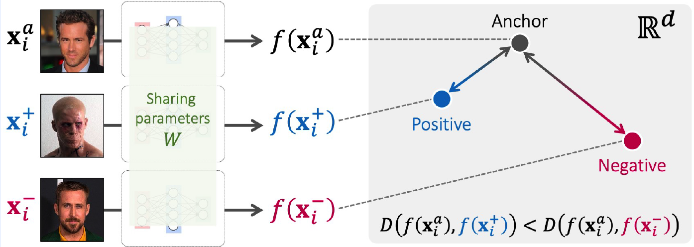
(3) Triplet Network
1) Notation
- anchor : \(x_i^a\)
- positive : \(x_i^{+}\)
- negative : \(x_i^{-}\)
2) Key idea
-
given anchor…
the distance between positive pair < distance between negative pair in the feature space
-
\(D\left(f\left(\boldsymbol{x}_{i}^{a}\right), f\left(\boldsymbol{x}_{i}^{+}\right)\right)+\delta<D\left(f\left(\boldsymbol{x}_{i}^{a}\right), f\left(\boldsymbol{x}_{i}^{-}\right)\right)\).
- \(\delta\) : margin
3) Triple Rank loss ( for triplet \(\left(\boldsymbol{x}_{i}^{a}, \boldsymbol{x}_{i}^{+}, \boldsymbol{x}_{i}^{-}\right)\) )
- \(L\left(W ; \boldsymbol{x}_{i}^{a}, \boldsymbol{x}_{i}^{+}, \boldsymbol{x}_{i}^{-}\right)=\max \left[0, \mid \mid f\left(\boldsymbol{x}_{i}^{a}\right), f\left(\boldsymbol{x}_{i}^{+}\right) \mid \mid _{2}^{2}- \mid \mid f\left(\boldsymbol{x}_{i}^{a}\right), f\left(\boldsymbol{x}_{i}^{-}\right) \mid \mid _{2}^{2}+\delta\right]\).
4) Details
After each data is passed through the NN….”L2 regularization”
Reason :
-
without normalization, margin becomes trivial!
-
ex) \(D\left(f\left(\boldsymbol{x}_{i}^{a}\right), f\left(\boldsymbol{x}_{i}^{+}\right)\right)+\delta\),
- \(\begin{gathered} \text {e.g., } 1,000,000+0.2<1,000,001 \end{gathered}\).
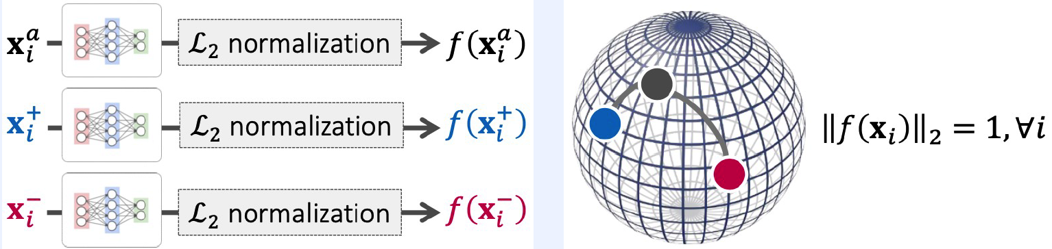
“Weight sharing” between both networks
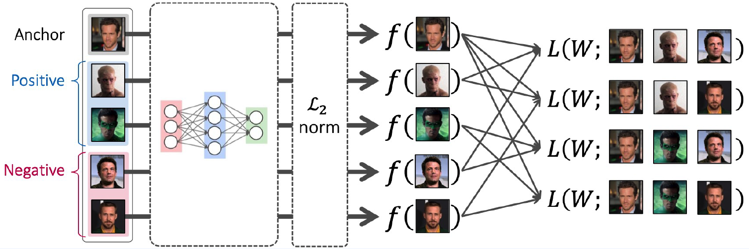
5) Sample Selection
infeasible to cover all pairs/triplets!
- (pairs) : \(O(N^2)\)
- (triplets) : \(O(N^3)\)
Difficulties
-
(1) TOO EASY pairs/triplets do not contribute to training
-
\(L\left(W ; \boldsymbol{x}_{i}^{a}, \boldsymbol{x}_{i}^{+}, \boldsymbol{x}_{i}^{-}\right)=\max \left[0, \mid \mid f\left(\boldsymbol{x}_{i}^{a}\right), f\left(\boldsymbol{x}_{i}^{+}\right) \mid \mid _{2}^{2}- \mid \mid f\left(\boldsymbol{x}_{i}^{a}\right), f\left(\boldsymbol{x}_{i}^{-}\right) \mid \mid _{2}^{2}+\delta\right]\),
-
if \(\mid \mid f\left(x_{i}^{a}\right), f\left(x_{i}^{+}\right) \mid \mid _{2}^{2}- \mid \mid f\left(x_{i}^{a}\right), f\left(x_{i}^{-}\right) \mid \mid _{2}^{2}+\delta<0\)
\(\rightarrow\) loss is 0
\(\rightarrow\) gradient is 0
\(\rightarrow\) no training!
-
-
-
(2) TOO HARD pairs/triplets could make training unstable
-
since \(\frac{\partial L}{\partial f\left(x_{i}^{-}\right)} \propto \frac{f\left(x_{i}^{a}\right)-f\left(x_{i}^{-}\right)}{ \mid \mid f\left(x_{i}^{a}\right)-f\left(x_{i}^{-}\right) \mid \mid ^{\prime}}\),
-
If TOO HARD negatives … and for hard negatives \(\mid \mid f\left(x_{i}^{a}\right), f\left(x_{i}^{-}\right) \mid \mid\) becomes too small
\(\rightarrow\) direction of gradients are NOT STABLE
-
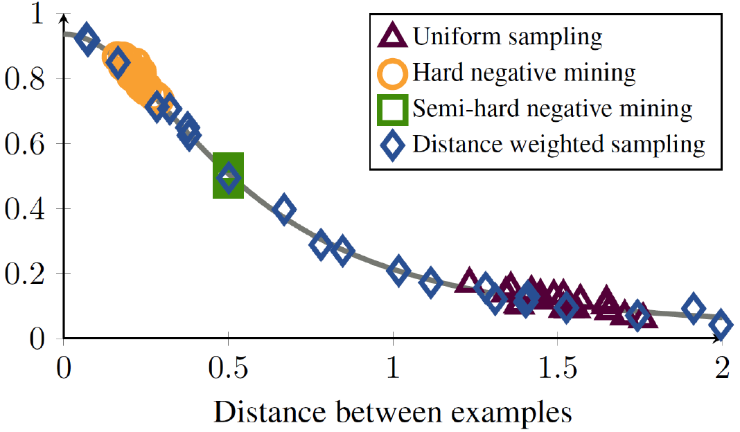
Uniform sampling
-
assuming an \(L_2\) normalized embedding space
\(\rightarrow\) distance between uniformly sampled points are “BIASED”
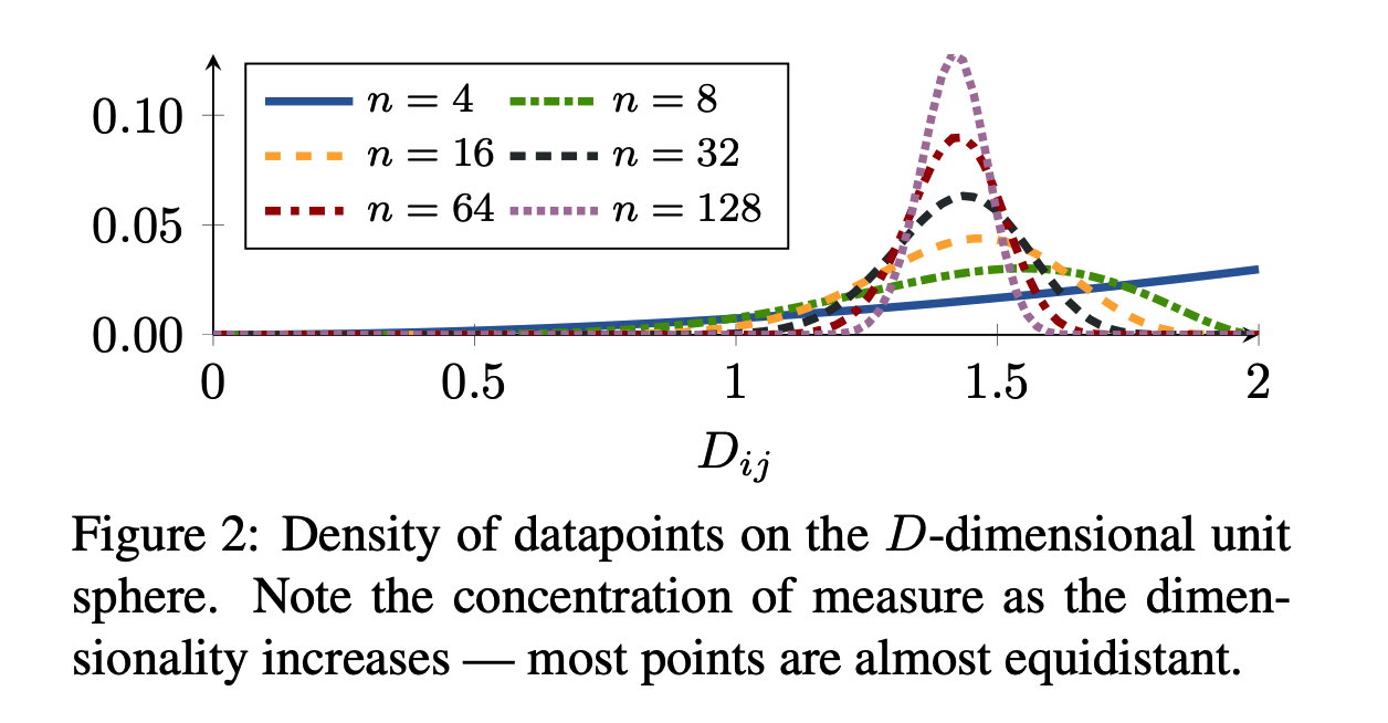
\(\rightarrow\) Need to select samples well!!
(4) Distance Weighted margin-based Loss
Solution of “Sample Selection problem” : Distance Weighted Sampling (DWS)
- correct the bias & control the variance
- sample negative examplesuniformly according to the DISTANCE from ANCHOR
\(P\left(n^{\prime}=n \mid a\right) \propto \min \left(\lambda, q^{-1}\left(D\left(f\left(x^{a}\right), f\left(x^{n^{\prime}}\right)\right)\right)\right)\),
- where \(q(D) \propto D^{d-2}\left[1-\frac{1}{4} d^{2}\right]^{\frac{n-3}{2}}\)
Empirical Analysis of DWS
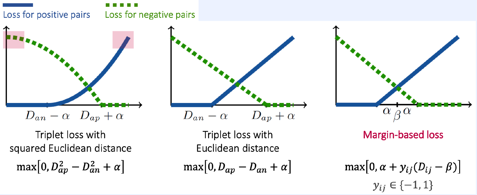
Margin-based loss
\(\ell^{\operatorname{margin}}(i, j):=\left(\alpha+y_{i j}\left(D_{i j}-\beta\right)\right)_{+}\).
- \(\beta\) : determines the boundary between positive and negative pairs
- \(\alpha\) : controls the margin of separation
- \(y_{i j} \in\{-1,1\}\).
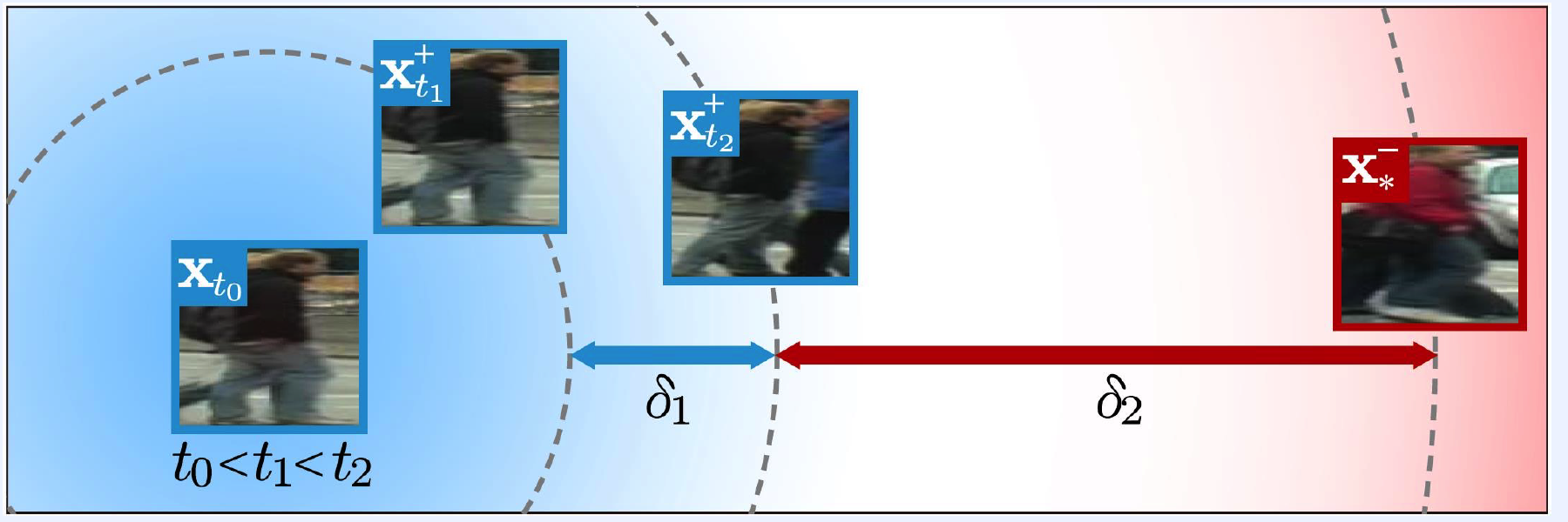
(5) Quadruplet Network
When is it used?
-
multi-object tracking : different relationships among positive samples,
accoring to their time indices
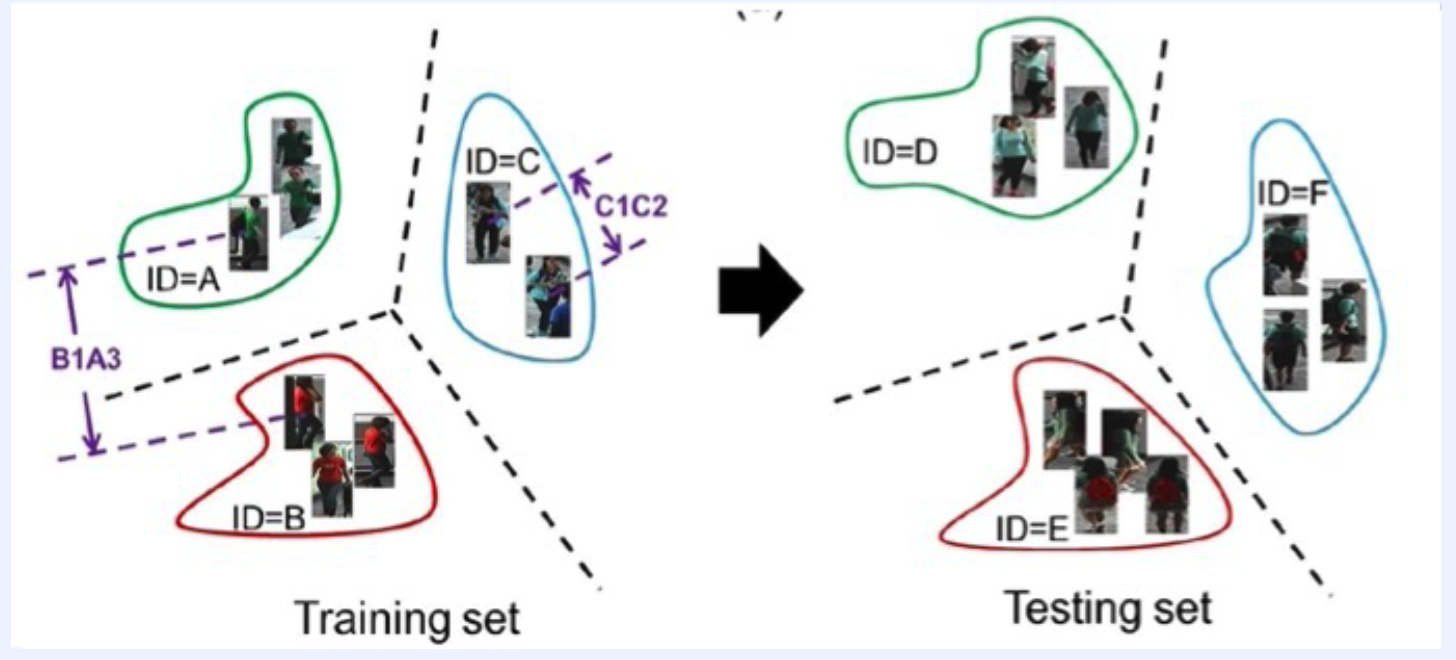
-
person re-identification : enlarging inter-class distances with additional constraints
1) Quadruplet Rank loss
linear combination of 2 Triplet Rank Losses
- \(L_{Q}\left(W ; \boldsymbol{x}_{i}^{a}, \boldsymbol{x}_{i}^{1}, \boldsymbol{x}_{i}^{2}, \boldsymbol{x}_{i}^{3}\right)=\alpha \cdot L_{T}^{1}\left(W ; \boldsymbol{x}_{i}^{a}, \boldsymbol{x}_{i}^{1}, \boldsymbol{x}_{i}^{2}\right)+\beta \cdot L_{T}^{2}\left(W ; \boldsymbol{x}_{i}^{a}, \boldsymbol{x}_{i}^{1}, \boldsymbol{x}_{i}^{3}\right)\).
\(\begin{aligned} &L_{Q}\left(W ; \boldsymbol{x}_{i}^{a}, \boldsymbol{x}_{i}^{t_{1}}, \boldsymbol{x}_{i}^{t_{2}}, \boldsymbol{x}_{i}^{-}\right) \\ &=\max \left[0, \mid \mid f\left(x_{i}^{a}\right), f\left(x_{i}^{t_{1}}\right) \mid \mid _{2}^{2}- \mid \mid f\left(x_{i}^{a}\right), f\left(x_{i}^{t_{2}}\right) \mid \mid _{2}^{2}+\delta_{1}\right] \\ &+\max \left[0, \mid \mid f\left(x_{i}^{a}\right), f\left(\boldsymbol{x}_{i}^{t_{2}}\right) \mid \mid _{2}^{2}- \mid \mid f\left(x_{i}^{a}\right), f\left(\boldsymbol{x}_{i}^{-}\right) \mid \mid _{2}^{2}+\delta_{2}\right] \end{aligned}\).
Notation
- \(\boldsymbol{x}_{i}^{a}\) : anchor
- \(\boldsymbol{x}_{i}^{t_{1}}, \boldsymbol{x}_{i}^{t_{2}}\) : positive ( time=1,2 respectively )
- \(\boldsymbol{x}_{i}^{-}\) : negative
2) Examples
\(\begin{aligned} &L_{Q}\left(W ; \boldsymbol{x}_{i}^{a}, \boldsymbol{x}_{i}^{t_{1}}, \boldsymbol{x}_{i}^{t_{2}}, \boldsymbol{x}_{i}^{-}\right) \\ &=\max \left[0, \mid \mid f\left(x_{i}^{a}\right), f\left(x_{i}^{t_{1}}\right) \mid \mid _{2}^{2}- \mid \mid f\left(x_{i}^{a}\right), f\left(x_{i}^{t_{2}}\right) \mid \mid _{2}^{2}+\delta_{1}\right] \\ &+\max \left[0, \mid \mid f\left(x_{i}^{a}\right), f\left(\boldsymbol{x}_{i}^{t_{2}}\right) \mid \mid _{2}^{2}- \mid \mid f\left(x_{i}^{a}\right), f\left(\boldsymbol{x}_{i}^{-}\right) \mid \mid _{2}^{2}+\delta_{2}\right] \end{aligned}\).
[ multi-object tracking ] Intepretation
- 1st term : positive samples closer in time should be closer to the anchor
- 2nd term : negative samples should be farther from the anchor than positive samples
[ person re-identification ] Intepretation
- 1st term : positive samples closer in time should be closer to the anchor
- 2nd term : inter-class distance > intra-class distance
(6) Nearest Neighbor Search
finding the nearest sample among training examples ( in a latent space )
(7) Applications
1) Image Retrieval
Content-based image retreieval
- nearest neighbor search in latent space
- works for unseen classes

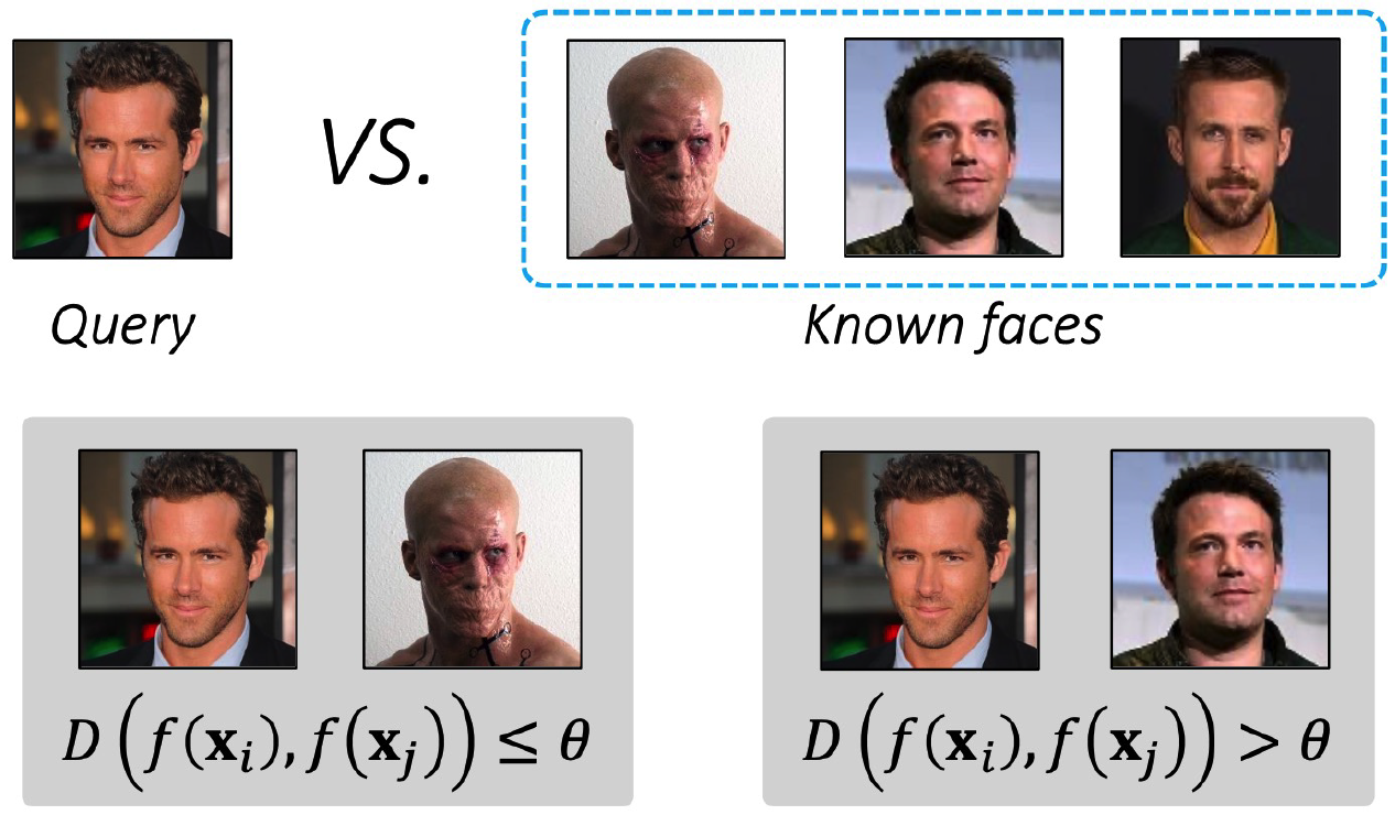
2) Face Verification
Task : decide if 2 face images are same/different
- apply a threshold to the distance ( in the latent space )
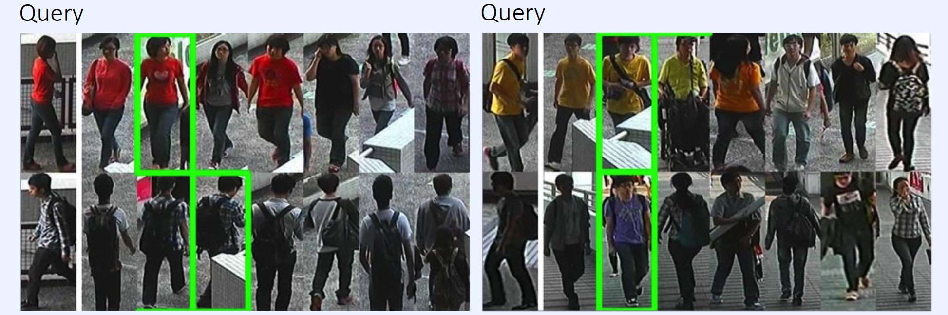
3) Person Re-identification
Task : identify people across different cameras
- works for unseen classes (=people)
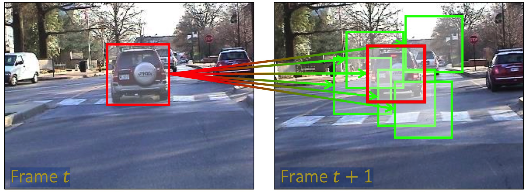
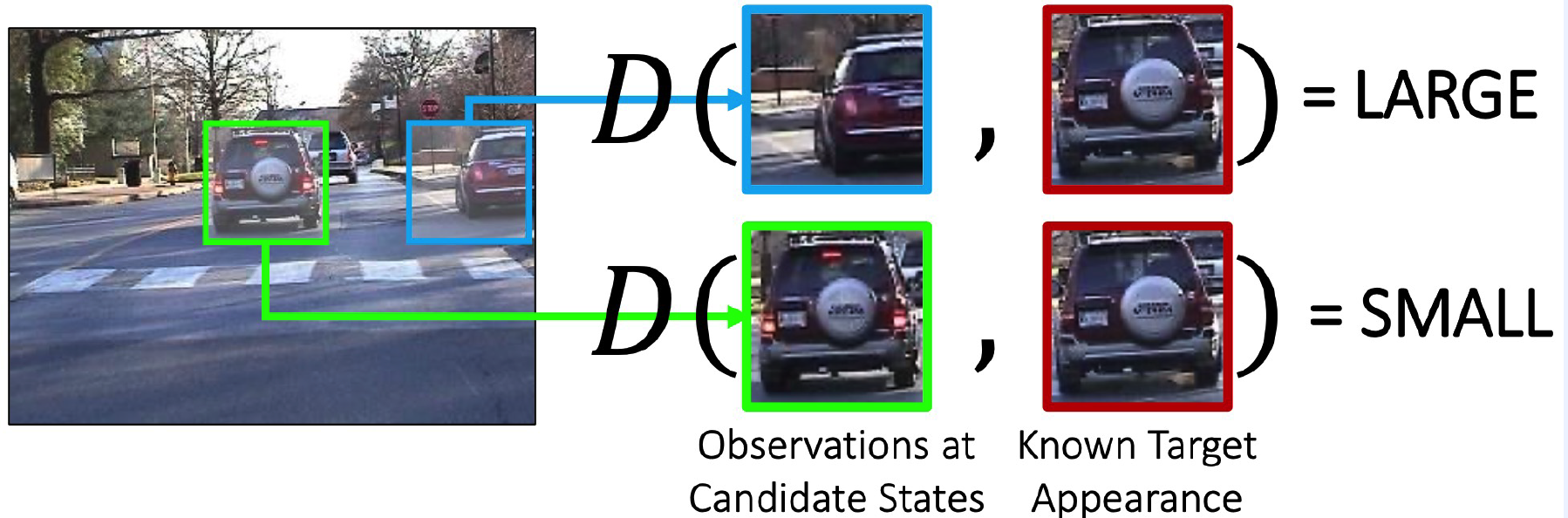
4) Online Visual Tracking
Task : track an object, which is manually annotated only in the 1st frame
- done by particle filtering + metric learning
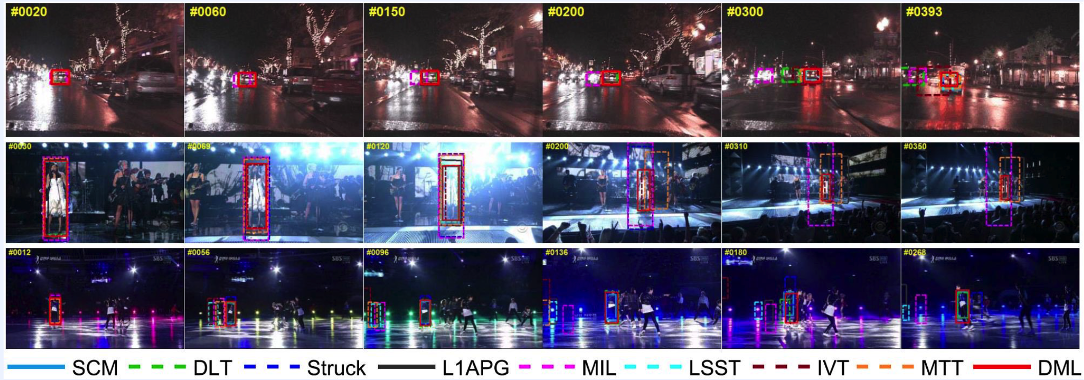
Particle Filtering?
-
Basic concept :
-
drawing random samples arount target location of previous time step
\(\rightarrow\) choose the most similar one!
-
similarity = inverse of distance
-
-
should be invariant to target object