[Explicit DGM] 01. Auto Encoders

[Explicit DGM] 01. Auto Encoders

( 참고 : KAIST 문일철 교수님 : 한국어 기계학습 강좌 심화 2)

Contents

1. Implicit vs Explicit distribution model
2. Deep Generative Model 소개
3. Autoencoder
4. Stacked Denoising Autoencoders

1. Implicit vs Explicit distribution model

Explicit : distribution에 대한 명시적 가정 O

• ex) VAE

Implicit : distribution에 대한 명시적 가정 X

• ex) GAN

2. Deep Generative Model 소개

Deep Generative Model (DGM)

• 딥러닝을 활용한 생성모델
• 새로운 데이터를 잘 생성해내기 위해, 딥러닝을 활용

DGM의 갈래

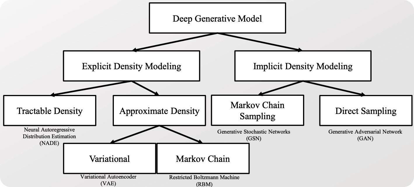
• 대표적인 DGM 모델 :
  • Explicit한 방법론에서는 VAE
  • Implicit한 방법론에서는 GAN

3. Autoencoder

• 목표 : input과 가장 유사한 output을 만들기

• 핵심 : 데이터의 핵심만을 잘 포착한 저차원으로 임베딩하기

일반적인 구조 : Encoder + Decoder

• Encoder : \(h(\cdot)\)
  • \(h(x)=g(a(x))=\sigma(b+W x)\).
• Decoder : \(o(\cdot)\)
  • \(\hat{x}=o(\hat{a}(x))=\sigma\left(c+W^{*} h(x)\right)\).
• notation
  • \(W,b\) : encoder의 파라미터
  • \(W^{*},c\) : decoder의 파라미터

Loss Function

• (1) CE ( Cross Entropy )
  • \(l(f(x))=-\sum_{d=1}^{D}\left(x_{d} \log \left(\hat{x}_{d}\right)+\left(1-x_{d}\right) \log \left(1-\hat{x}_{d}\right)\right)\).
• (2) MSE ( Mean Squared Error )
  • \(l(f(x))=\frac{1}{2} \sum_{d=1}^{D}\left(\hat{x}_{d}-x_{d}\right)^{2}\).

위 모델에서, encoder & decoder을 NN을 사용하면, DEEP generative model (DGM)이 된다.

4. Stacked Denoising Autoencoders

DENOISING autoencoder

• 이름에서도 알 수 있 듯, 노이즈를 제거 ( 보다 엄밀하겐, 노이즈에 robust한 ) autoencoder이다.

• 이러한 denoising autoencoder을 여러개의 MLP를 쌓아서 만든 것이 Stacked Denoising Autoencoder 이다.

Autoencoder vs DENOISING autoencoder

• Input의 차이
  • AE : \(x\)
  • DAE : \(x\) + noise ( = \(\tilde{x}\) )
• 그 외에는 전부 동일하다.

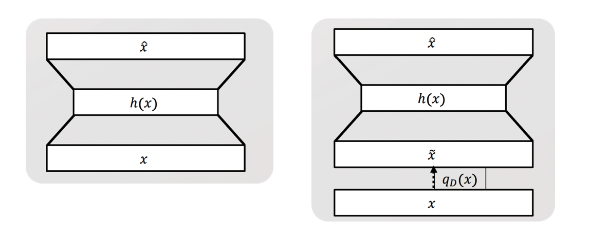
Noise Process : input에 noise를 더해주는 과정

• \(\tilde{x}=q_{D}(x)\).
• 예시 )
  • Additive Gaussian noise : \(q_{D}(x)=x+\epsilon, \epsilon \sim N\left(\mu_{D}, \Sigma_{D}\right)\)
  • Masking noise : \(q_{D}(x)=x \epsilon_{d}, \epsilon_{d} \sim \operatorname{Bernoulli}(p)\)

수식도, 위의 input이 다르다는 점을 제외하고는 전부 동일하다!

일반적인 구조 : Encoder + Decoder

• Encoder : \(h(\cdot)\)
  • \(h(x)=g(a(\tilde{x}))=\sigma(b+W \tilde{x})\).
• Decoder : \(o(\cdot)\)
  • \(\hat{x}=o(\hat{a}(\tilde{x}))=\sigma\left(c+W^{*} h(\tilde{x})\right)\).

Loss Function

• (1) CE ( Cross Entropy )
  • \(l(f(x))=-\sum_{d=1}^{D}\left(x_{d} \log \left(\hat{x}_{d}\right)+\left(1-x_{d}\right) \log \left(1-\hat{x}_{d}\right)\right)\).
• (2) MSE ( Mean Squared Error )
  • \(l(f(x))=\frac{1}{2} \sum_{d=1}^{D}\left(\hat{x}_{d}-x_{d}\right)^{2}\).

요약

• input이 동일하더라도, noise가 더해지는 과정때문에 서로 다른 output이 다를 수 있다 ( stochasticity 부여 )
• 하지만, output 생성 과정은 여전히 deterministic하다. input만 stochastic 할 뿐이다.