(paper 92) Diffusion-based TS Imputation and Forecasting with SSSM

Diffusion-based TS Imputation and Forecasting with SSSM

Contents

1. Abstract
2. Introduction
3. SSSD models for TS imputation
   1. TS imputation
   2. Diffusion models
   3. State space models
   4. Proposed approaches

0. Abstract

Imputation of missing values

Proposes SSSD

• Imputation model
• relies on 2 emerging technologies
  • (1) (conditional) Diffusion models … as generative model
  • (2) Structured state space models (SSSM) ….. as internal model architecture
    • suited to capture long-term dependencies in TS

Experiment : “probabilistic” imputation and forecasting

1. Introduction

Focus on TS as a data modality, where missing data is particularly prevalent

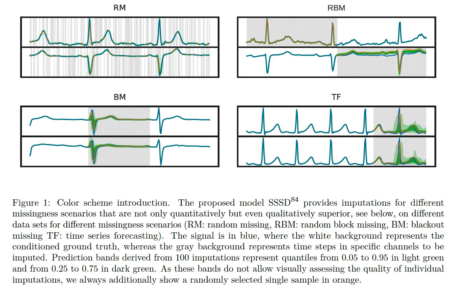
Different missingness scenarios

• ex) TS forecasting = missingness at the end of sequence ( = future )

“PROBABILISTIC” imputation methods

• single imputation (X)
• samples of different plausible imputations (O)

TS imputation

Review : (Osman et al., 2018)

• Statistical methods (Lin & Tsai, 2020)
• AR models (Atyabi et al., 2016; Bashir & Wei, 2018)
• Generative models

However, many existing models remain limited to the RM (random missing) scenario

This paper : Address these shortcomings,

• by proposing a new GENERATIVE-model-based approach for TS imputation.

Details:

• (1) Diffusion Models

• (2) Structured State Space Models

  ( instead of dilated CNN, transformer layers )

  • particularly suited to handling long-term-dependencies

Contributions

1. Combination of
   • SSM as ideal building blocks to capture long-term dependencies
   • (Conditional) diffusion models for generative modeling
2. Modifications to the contemporary diffusion model architecture DiffWave
3. Experiments

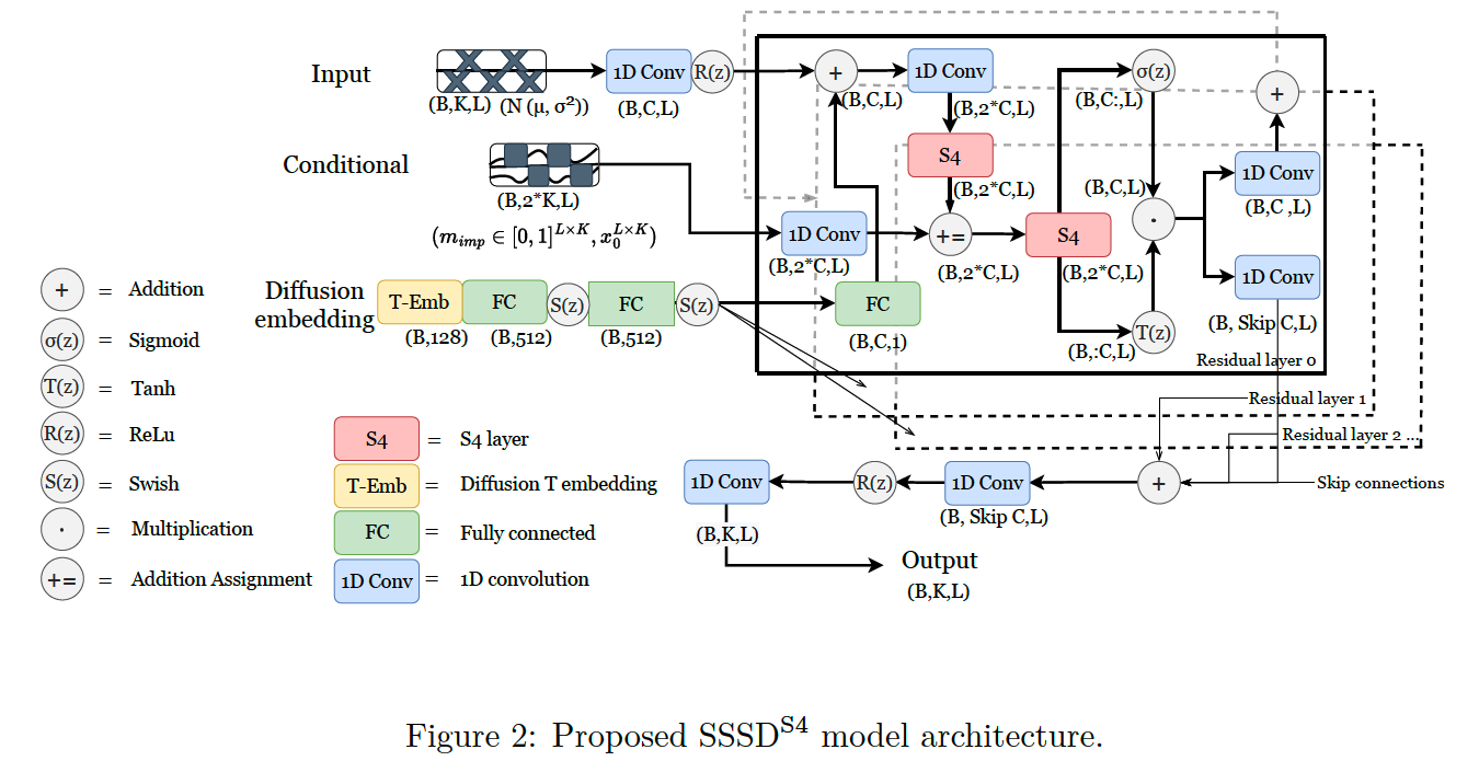
2. Structured state space diffusion (SSSD) models for time series imputation

(1) TS imputation

Notation

• \(x_0\) : data sample with shape \(\mathbb{R}^{L \times K}\)
• Imputation targets : specified in terms of binary masks
  • i.e., \(m_{\mathrm{imp}} \in\{0,1\}^{L \times K}\),
    • 1 = condition
    • 0 = target to be imputed
  • if missing value also in the input … additionally requires a mask \(m_{\mathrm{mvi}}\)

Missingness scenarios

• MCAR : missing completely at random ( THIS PAPER )
  • missingness pattern does not depend on feature values
• MAR : missing at random
  • may depend on observed features
• RBM : random block missing
  • may depend also on ground truth values of the features to be imputed

Random missing (RM)

• zero-entries of \(m_{\mathrm{imp}}\) are sampled randomly
• thie paper : consider single time steps for RM instead of blocks of consecutive time steps.

(2) Diffusion models

Learn a mapping from a latent space to the original signal space,

by learning to remove noise in a backward process that was added sequentially in a Markovian fashion during forward process

[ UNconditional case ]

Forward Process

\(q\left(x_1, \ldots, x_T \mid x_0\right)=\prod_{t=1}^T q\left(x_t \mid x_{t-1}\right)\).

• where \(q\left(x_t \mid x_{t-1}\right)=\mathcal{N}\left(\sqrt{1-\beta_t} x_{t-1}, \beta_t \mathbb{1}\right)\left[x_t\right]\)

  • \(\beta_t\) = noise level (fixed or learnable)

    ( ex. 0.0001 )

\(\begin{aligned} \mathbf{x}_t & =\sqrt{\alpha_t} \mathbf{x}_{t-1}+\sqrt{1-\alpha_t} \epsilon_{t-1} \\ & =\sqrt{\alpha_t \alpha_{t-1}} \mathbf{x}_{t-2}+\sqrt{1-\alpha_t \alpha_{t-1}} \bar{\epsilon}_{t-2} \\ & =\ldots \\ & =\sqrt{\bar{\alpha}_t} \mathbf{x}_0+\sqrt{1-\bar{\alpha}_t} \boldsymbol{\epsilon} \end{aligned}\).

• where \(\alpha_t=1-\beta_t\) and \(\bar{\alpha}_t=\prod_{i=1}^t \alpha_i\)

  ( + we know \(\beta_t\) in advance! )

\(q\left(\mathbf{x}_t \mid \mathbf{x}_0\right) = \mathcal{N}\left(\mathbf{x}_t ; \sqrt{\bar{\alpha}_t} \mathbf{x}_0,\left(1-\bar{\alpha}_t\right) \mathbf{I}\right)\).

Backward Process

\(p_\theta\left(x_0, \ldots, x_{t-1} \mid x_T\right)=p\left(x_T\right) \prod_{t=1}^T p_\theta\left(x_{t-1} \mid x_t\right)\).

• where \(x_T \sim \mathcal{N}(0, \mathbb{1})\).
• \(p_\theta\left(x_{t-1} \mid x_t\right)\) = assumed as normal-distributed (with diagonal covariance matrix)

Under particular parametrization of \(p_\theta\left(x_{t-1} \mid x_t\right)\) ….

Reverse process can be trained using …

\(L=\min _\theta \mathbb{E}_{x_0 \sim \mathcal{D}, \epsilon \sim \mathcal{N}(0, \mathbb{1}), t \sim \mathcal{U}(1, T)} \mid \mid \epsilon-\epsilon_\theta\left(\sqrt{\alpha_t} x_0+\left(1-\alpha_t\right) \epsilon, t\right) \mid \mid _2^2\).

• \(\epsilon_\theta\left(x_t, t\right)\) : parameterized using a NN

  ( = score-matching techniques )

• can be seen as a weighted variational bound on the NLL that down-weights the importance of terms at small \(t\), i.e., at small noise levels.

[ Conditional case ]

Backward process is conditioned on additional information

• i.e. \(\epsilon_\theta=\epsilon_\theta\left(x_t, t, c\right)\),

Condition?

= the concatenation of input & imputation mask

• i.e., \(c=\operatorname{Concat}\left(x_0 \odot\left(m_{\mathrm{imp}} \odot m_{\mathrm{mvi}}\right),\left(m_{\mathrm{imp}} \odot m_{\mathrm{mvi}}\right)\right)\),
  • \(m_{\mathrm{imp}}\) : imputation mask
  • \(m_{\mathrm{mvi}}\) : missing value mask

2 different setups

• \(D_0\) : apply the diffusion process to the full signal

• \(D_1\) : apply the diffusion process to the regions to be imputed only

( Still, evaluation of the loss function is only supposed to be on the input values for which ground truth information is available, i.e., where \(m_{\mathrm{mvi}}=1\). )

(3) State space models (SSM)

Linear state space transition equation

• connecting a 1-D input \(u(t)\) to a 1-d output \(y(t)\)

  via a \(N\)-D hidden state \(x(t)\).

• \(x^{\prime}(t)=A x(t)+B u(t) \text { and } y(t)=C x^{\prime}(t)+D u(t)\).

Relation between input & output

= can be written as a convolution operation

Ability to capture long-term dependencies

= relates to a particular initialization of \(A \in \mathbb{R}^{N \times N}\) according to HiPPO theory

(4) Proposed approaches