(paper) GCN ; a comprehensive review

GCN ; a comprehensive review

Contents

1. Abstract
2. Introduction
3. Notations & Preliminaries
4. Graph Fourier Transform
5. Graph Filtering
6. Spectral GCNs
7. Spatial GCNs

Abstract

Challenges of Graph

• (1) many types of data are not originally structured as graphs
• (2) underlying connvectivity patterns are complex & diverse

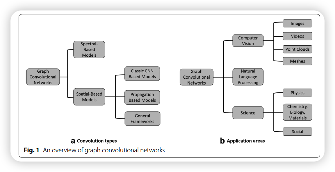
This paper : review on GCN

• (1) group the exisiting GCN models into 2 categories
• (2) categorize different GCN, according to applications

1. Introduction

2. Notations & Preliminarries

Undirected graph : \(\mathcal{G}=\{\mathcal{V}, \mathcal{E}, \mathbf{A}\}\)

• \(\mid \mathcal{V} \mid =n\) & \(\mid \mathcal{E} \mid =m\)

Degree matrix : \(\mathbf{D}\)

• \(\mathbf{D}(i, i)=\sum_{j=1}^{n} \mathbf{A}(i, j)\).

Laplacian matrix : \(\mathbf{L}=\mathbf{D}-\mathbf{A}\)

Symmetrically Normalized Laplacian matrix : \(\tilde{\mathbf{L}}=\mathbf{I}-\mathbf{D}^{-\frac{1}{2}} \mathbf{A D} \mathbf{D}^{-\frac{1}{2}}\)

Graph Signal ( on nodes ) : \(\mathbf{x} \in \mathbb{R}^{n}\)

• \(\mathbf{x}(i)\) : single value on node \(i\)

Node attribute matrix : \(\mathbf{X} \in \mathbb{R}^{n \times d}\)

• columns of \(\mathbf{X}\) are the \(d\) signals of the graph.

3. Graph Fourier transform

classic Fourier transform ( of 1-D signal \(f\) ) : \(\hat{f}(\xi)=\left\langle f, e^{2 \pi i \xi t}\right\rangle\)

• \(\xi\) : frequency
• \(\hat{f}\) : spectral domain
• complex exponential : eigenfunction of the Laplace operator

Laplacian matrix \(\mathbf{L}\) :

• Laplace operator defined on a graph

  ( eigenvector of \(\mathbf{L}\) associated with its corresponding eigenvalue is an analog to the complex exponential at a certain frequency )

• not only \(L\), but also, \(\tilde{\mathbf{L}}\) can be used

Eigenvalue decompositon of \(\tilde{\mathbf{L}}\) : \(\tilde{\mathbf{L}}=\mathbf{U} \boldsymbol{\Lambda} \mathbf{U}^{T}\)

• \(l^{th}\) column of \(\mathbf{U}\) : eigen vector \(u_l\)
  • eigen value : \(\boldsymbol{\Lambda}(l, l)\) ( = \(\lambda_{l})\)
• the, Fourier transform of graph signal \(\mathbf{x}\) :
  • \(\hat{\mathbf{x}}\left(\lambda_{l}\right)=\left\langle\mathbf{x}, \mathbf{u}_{l}\right\rangle=\sum_{i=1}^{n} \mathbf{x}(i) \mathbf{u}_{l}^{*}(i)\).
• inverse graph Fourier Transform :
  • \(\mathbf{x}(i)=\sum_{l=1}^{n} \hat{\mathbf{x}}\left(\lambda_{l}\right) \mathbf{u}_{l}(i)\).

\(\rightarrow\) those are all SPECTRAL domain

4. Graph Filtering

LOCALIZED OPERATION on graph signals

• one can localize a graph signal, in its (1) vertex domain or (2) spectral domain

(1) Frequency Filtering

( classical signal ) convolution with the filter signal in the time domain

( in graph ) due to the irregular structure of the graphs……

• graph convolution in the vertex domain is not as straightforward as the classic one

( classical signal ) convolution in time domain

= IFT of the multiplication between the spectral representation of 2 signals

\(\rightarrow\) Therefore, the spectral graph convolution is defined analogously as:

\(\left(\mathbf{x} *_{\mathcal{G}} \mathbf{y}\right)(i)=\sum_{l=1}^{n} \hat{\mathbf{x}}\left(\lambda_{l}\right) \hat{\mathbf{y}}\left(\lambda_{l}\right) \mathbf{u}_{l}(i)\).

• \(\hat{\mathbf{x}}\left(\lambda_{l}\right) \hat{\mathbf{y}}\left(\lambda_{l}\right)\) : filtering in the spectral domain

Frequency Filtering of signal \(\mathbf{x}\), on graph \(\mathcal{G}\) , with filter \(\mathbf{y}\) :

• same as equation above!

• can be rewritten as…

  \(\mathbf{x}_{\text {out }}=\mathbf{x} *_{\mathcal{G}} \mathbf{y}=\mathbf{U}\left[\begin{array}{cc} \hat{\mathbf{y}}\left(\lambda_{1}\right) & 0 \\ & \ddots \\ 0 & \hat{\mathbf{y}}\left(\lambda_{n}\right) \end{array}\right] \mathbf{U}^{T} \mathbf{x}\).

(2) Vertex Filtering

graph filtering of signal \(\mathbf{x}\) in vertex domain :

• generally defined as LINEAR COMBINATION of signal components in the neighbors

Vertex filtering of singal \(\mathbf{x}\) at node \(i\) :

• \(\mathbf{x}_{\text {out }}(i)=w_{i, i} \mathbf{x}(i)+\sum_{j \in \mathcal{N}(i, K)} w_{i, j} \mathbf{x}(j)\). ( for \(K\) hop neighborhood )

Using a \(K\) polynomial filter, frequency filtering can be interpreted from vertex filtering

5. Spectral GCNs

categorize GCN into..

• (1) SPECTRAL based methods

  ( = method taht starts with constructing the frequency filtering )

• (2) SPATIAL based methods

(1) Bruna et al [32]

Details

• first notable spectral based GCN

• contains several spectral convolutional layers

  • input : \(\mathbf{X}^{p}\) …. size : \(n \times d_p\) ( \(p\) : index of layer )
  • output : \(\mathbf{X}^{p+1}\) ….. size : \(n \times d_{p+1}\)

  \(\mathbf{X}^{p+1}(:, j)=\sigma\left(\sum_{i=1}^{d_{p}} \mathbf{V}\left[\begin{array}{cc} \left(\boldsymbol{\theta}_{i, j}^{p}\right)(1) & 0 \\ & \ddots \\ 0 & \left(\boldsymbol{\theta}_{i, j}^{p}\right)(n) \end{array}\right] \mathbf{V}^{T} \mathbf{X}^{p}(:, i)\right), \quad \forall j=1, \cdots, d_{p+1}\).

• \(\boldsymbol{\theta}_{i, j}^{p}\) : vector of learnable parameters ( at \(p\) th layer )
• each column of \(\mathbf{V}\) is the eigenvector of \(\mathbf{L}\)

Limitations

• (1) eigenvector matrix \(\mathbf{V}\) requires the explicit computation of the eigenvalue decomposition of the graph Laplacian matrix

  \(\rightarrow\) \(O\left(n^{3}\right)\) time complexity

• (2) though the eigenvectors can be pre-computed…

  the time complexity of equation above is still \(O\left(n^{2}\right)\)

• (3) there are \(O(n)\) parameters to be learned in

Solution : use a rank-\(r\) approximation of EV decomposition

• use first \(r\) eigenvectors of \(\mathbf{V}\)
  • have the most smooth geometry of the graph
• reduce the number of parameters of each filter to O(1)

However, the computational complexity and the localization power still hinder learning better representations of the graphs.

(2) ChebNet

Uses \(K\) polynomial filters in conv layers for localization

• \(\hat{\mathbf{y}}\left(\lambda_{l}\right)=\sum_{k=1}^{K} \theta_{k} \lambda_{l}^{k}\).
• \(K\)-polynomial filters :
  • achieve a good localization in the vertex domain
  • by integrating the node features within the \(K\) hop neighborhood
• number of trainable parameters \(O(K) \rightarrow O(1)\)
• to further reduce the computational complexity, the Chebyshev polynomial approximation is used to compute the spectral graph convolution

Chebyshev polynomial \(T_k(x)\) of order \(k\)

• can be recursively computed by \(T_{k}(x)=2 x T_{k-1}(x)-T_{k-2}(x)\)
• where \(T_{0}=1, T_{1}(x)=x\).

etc

• normalize the filters by \(\tilde{\lambda}_{l}=2 \frac{\lambda_{l}}{\lambda_{\operatorname{mav}}}-1\)

  \(\rightarrow\) make the scaled eigenvalues lie within \(\lfloor-1,1\rfloor\)

Summary

\(\mathbf{X}^{p+1}(:, j)=\sigma\left(\sum_{i=1}^{d_{p}} \sum_{k=0}^{K-1}\left(\boldsymbol{\theta}_{i, j}^{p}\right)(k+1) T_{k}(\tilde{\mathbf{L}}) \mathbf{X}^{p}(:, i)\right), \quad \forall j=1, \ldots, d_{p+1}\).

• \(\boldsymbol{\theta}_{i, j}^{p}\) : \(K\)-dim parameter vectorr

(3) Kipf et al [37]

semi-supervised node classification

• (change 1) truncate Chebyshev polynomial to first order ( \(K=2\) )
• (change 2) set \((\boldsymbol{\theta})_{i, j}(1)=-(\boldsymbol{\theta})_{i, j}(2)=\theta_{i, j}\).
• (change 3) relax \(\lambda_{max}=2\)

Simplified convolution layer : \(\mathbf{X}^{p+1}=\sigma\left(\tilde{\mathbf{D}}^{-\frac{1}{2}} \tilde{\mathbf{A}} \tilde{\mathbf{D}}^{-\frac{1}{2}} \mathbf{X}^{p} \mathbf{\Theta}^{p}\right)\)

• where \(\tilde{\mathbf{A}}=\mathbf{I}+\mathbf{A}\) & \(\tilde{\mathbf{D}}\) is the diagonal degree matrix of \(\tilde{\mathbf{A}}\),

(4) FastGCN

improves GCN, by enabling efficient minibatch training

6. Spatial GCNs

Spectral GCN

• relies on the specific eigenfunctions of Laplacian matrix

  \(\rightarrow\) not easy to transfer to graph with different structure

Spatial GCN

• graph filtering in vertex domain : convolution can be alternatively generalized to some aggregations of graph signals within the node neighborhood

categorize Spatial GCN into..

• (1) classic CNN-based models
• (2) propagation-based models
• (3) related general frameworks

(1) classic CNN-based models

Basic properties of grid like data

• (1) the number of neighboring pixels for each pixel is fixed
• (2) the spatial order of scanning images is naturally determined

but in graph data….

• neither the number of neighboring units nor the spatial order among them is fixed

Many works have been proposed to build GCN directly upon the classic CNNs

a) PATCHY-SAN

step 1) determines the nodes ordering

• by a given graph labeling approach such as centrality-based methods
• (e.g., degree, PageRank, betweenness, etc.)
• Then selects a fixed-length sequence of nodes

step 2) fixed-size neighborhood for each node is constructed

• to address the issue of arbitrary neighborhood size of nodes

step 3) neighborhood graph is normalized

• nodes of similar structural roles are assigned similar relative positions

step 4) representation learning with classic CNNs

Limitations : spatial order of nodes is determined by the given graph labeling approach

\(\rightarrow\) often solely based on graph structure

\(\rightarrow\) lacks the learning flexibility and generality to a broader range of applications.

b) LGCN

( \(\leftrightarrow\) PATCHY SAN : order nodes by structural inforrmation )

LGCN : proposed to tansfomr the irregular graph data to grid-like data, by using..

• (1) structural information
• (2) input feature map of \(p\)-th layer

Steps

• step 1) stacks input feature map of node \(u\)’s neighbors into a single matrix \(\mathbf{M} \in \mathbb{R}^{ \mid \mathcal{N}(u) \mid \times d_{p}}\)

• step 2) for each column of \(\mathbf{M}\) , the first \(r\) largest values are preserved and form a new matrix \(\tilde{\mathbf{M}} \in \mathbb{R}^{r \times d_{p}}\).

• step 3) “input feature map” & “strutural information”

  \(\rightarrow\) transformed to an 1-D grid like data \(\tilde{\mathbf{X}}_{p} \in \mathbb{R}^{n \times(r+1) \times d_{p}}\)

• step 4) apply 1-D CNN to \(\tilde{\mathbf{X}}^{p}\)

• step 5) get new node representation \(\mathbf{X}^{p+1}\)

(2) propagation-based models

ex) Graph convolution for node \(u\) at the \(p\)th layer :

• \(\mathbf{x}_{\mathcal{N}(u)}^{p}=\mathbf{X}^{p}(u,:)+\sum_{v \in \mathcal{N}(u)} \mathbf{X}^{p}(v,:)\).

• \(\mathbf{X}^{p+1}(u,:)=\sigma\left(\mathbf{x}_{\mathcal{N}(u)}^{p} \boldsymbol{\Theta}_{ \mid \mathcal{N}(u) \mid }^{p}\right)\).

  • where \(\boldsymbol{\Theta}_{ \mid \mathcal{N}(u) \mid }^{p}\) : weight matrix for nodes with SAME DEGREE

  • problem : inappropriate with LARGE graphs

a) DCNN ( Diffusion based GCN )

\(k\)-step diffusion :

• \(k\) th power of transition matrix \(\mathbf{P}^{k}\) ( where \(\mathbf{P}=\mathbf{D}^{-1} \mathbf{A}\) )

Diffusion-convolution operation :

• \(\mathbf{Z}(u, k, i)=\sigma\left(\boldsymbol{\Theta}(k, i) \sum_{v=1}^{n} \mathbf{P}^{k}(u, v) \mathbf{X}(v, i)\right)\).

  • \(i\) th output feature of node \(u\) aggregated based on \(\mathbf{P}^{k}\)

  • \(K\)-th power of transition matrix \(\rightarrow\) \(O(n^2K\) ) computational complexity

    ( also inappropriate for LARGE graphs )

b) MoNet

generic GCN framework

• design a universe patch operator, which integrates the signals within the node neighborhood

Details : for node \(i\) & neighbor \(j \in \mathcal{N}(i)\),

• step 1) define a \(d\)-dimensional pseudo-coordinates \(\mathbf{u}(i, j)\)

• step 2) feed it into \(P\) learnable kernel functions \(\left(w_{1}(\mathbf{u}), \ldots, w_{P}(\mathbf{u})\right)\)

• step 3) patch operator is formulated as …

  • \[D_{p}(i)=\sum_{j \in \mathcal{N}(i)} w_{p}(\mathbf{u}(i, j)) \mathbf{x}(j), p=1, \ldots, P\]

    (. where \(\mathbf{x}(j)\) is the signal value at the node \(j\) )

• step 4) GCN in spatial domain

  • \(\left(\mathbf{x} *_{s} \mathbf{y}\right)(i)=\sum_{l=1}^{p} \mathbf{g}(p) D_{p}(i) \mathbf{x}\).

Diverse selection of \(\mathbf{u}(i, j)\) and the kernel function \(w_{p}(\mathbf{u})\),

\(\rightarrow\) many existing GCNs are specific case of MoNet.

( ex. Spline CNN : use \(B\)-splines )

c) graphs with edge attributes

• edge-conditioned convolution (ECC) operation

d) GraphSAGE

aggregation-based inductive representation learning model

Details : for a node \(u\)..

• step 1) aggregates the reprsentation vectors of all its immediate neighbors in the current layer with some learnable aggregator
• step 2) concatenate representation vector & aggregated representation
• step 3) feed them to FC layer

\(p\)-th convlutional layer in GraphSAGE :

• \(\mathbf{x}_{\mathcal{N}(u)}^{p} \leftarrow \operatorname{AGGREGATE}_{p}\left(\left\{\mathbf{X}^{p}(v,:), \forall v \in \mathcal{N}(u)\right\}\right)\),
• \(\mathbf{X}^{p+1}(u,:) \leftarrow \sigma\left(\operatorname{CONCAT}\left(\mathbf{X}^{p}(u,:), \mathbf{x}_{\mathcal{N}(u)}^{p}\right) \boldsymbol{\Theta}^{p}\right)\).

several choices of the aggregator functions

• mean aggregator
• LSTM aggregator
• pooling aggregator

has been shown that a two-layer graph convolution model often achieves the best performance in GCN & GraphSAGE

( do not make it TOO DEEP )

e) Jumping Knowledge Network

• mitigate DEEP LAYER issue
• borrow idea from ResNet
• adaptively select the aggregations from the different convolution layers
  • selectively aggregate the intermediate representations for each node independently

layer-wise aggregators

• concatenation aggregator
• max-pooling aggregator
• LSTM-attention aggregator

also admits the combination with the other existing GNN models

(3) related general frameworks

• Gated GNN
• GAT

a) earliest graph neural networks is [66]

Notation

• parametric local transition : \(f\)
• local output function : \(g\)
• input attributes of node \(u\) : \(\mathbf{X}^{0}(u,:)\)
• edge ~ : \(\mathbf{E}_{u}\)

Local transition function

• \(\mathbf{H}(u,:)=f\left(\mathbf{X}^{0}(u,:), \mathbf{E}_{u}, \mathbf{H}(u,:), \mathbf{X}^{0}(\mathcal{N}(u),:)\right)\).

Local output function

• \(\mathbf{X}(u,:)=g\left(\mathbf{X}^{0}(u,:), \mathbf{H}(u,:)\right)\).

( where \(\mathbf{H}(u,:), \mathbf{X}(u,:)\) are the hidden state and output representation of node \(u\) )

b) MPNNs ( Message Passing NN )

generalize many variants of GNN (ex. GCN, gated GNN )

2 phase model

• step 1) message passing phase
  • runs node aggregations for \(P\) steps
  • each step : 2 functions
    • (1) message function : \(\mathbf{H}^{p+1}(u,:)=\sum_{v \in \mathcal{N}(u)} M^{p}\left(\mathbf{X}^{p}(u,:), \mathbf{X}^{p}(v,:), \mathbf{e}_{u, v}\right)\)
    • (2) update function : \(\mathbf{X}^{p+1}(u,:)=U^{p}\left(\mathbf{X}^{p}(u,:), \mathbf{H}^{p+1}(u,:)\right)\)
• step 2) readout phase
  • computes the feature vector for the whole graph
  • \[\hat{\mathbf{y}}=R\left(\left\{\mathbf{X}^{P}(u,:) \mid u \in \mathcal{V}\right\}\right)\]