
Chapter 5. Aggregation
( 참고 : https://www.youtube.com/watch?v=JtDgmmQ60x8&list=PLGMXrbDNfqTzqxB1IGgimuhtfAhGd8lHF )
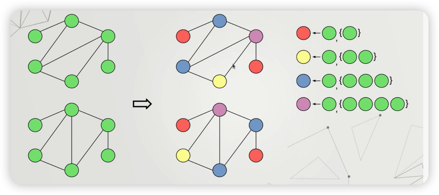
1) WL Isomporhpism Test
요약 : 2개의 그래프가 동일한지 확인하는 테스트
Step 1) 우선, 이웃 노드의 개수가 1개/2개/…./n개인 노드를 각각 다른색으로 칠한다
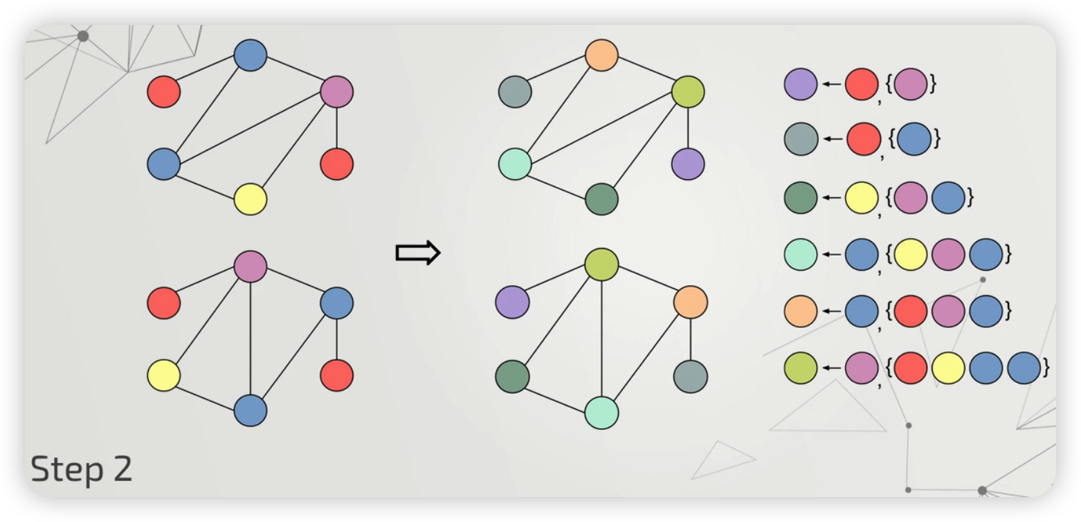
Step 2) 이번에는, 이웃 노드의 색깔까지 고려하여, 다른 색으로 칠한다
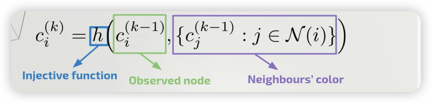
위의 간단한 과정을, 수식으로 나타내면 아래와 같다.
- (참고) 이때, “고유한 색을 칠하는 함수”를 injective function으로 볼 수 있다.
이때, 이러한 의문점이 들 수 있다.
과연, 우리는 위의 WL isomorphism test를 수행할 수 있는 (그만큼 복잡한/powerful한) GNN을 만들 수 있는가?
\(\rightarrow\) 이에 대한 해답으로 GIN (Graph Isomorphism Network)가 등장한다
2) GIN (Graph Isomorphism Network)
Notation
- \(G\) & \(G’\) : two NON isomorhpic graphs
- \(\mathcal{A}\) : GNN ( \(G \rightarrow R^d\) )
Goal
- construct GNN, such that \(\left\{h_{i}: i \in V(G)\right\}\) and \(\left\{h_{j}: j \in V\left(G^{\prime}\right)\right\}\) differ
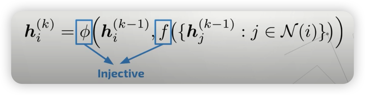
Updating equation
- 따라서, 마찬가지로 아래에서도 \(\phi\) 와 \(f\) 는 injective function 이어야 한다.
이때, 우리는 injective function의 특징에 대해 살펴보아야 한다.
그 중 하나의 특징은, multiset에 대한 injective function은 아래와 같이 decompose ( = sum-decomposition ) 될 수 있다는 것이다.
- \(g(X)=\phi\left(\sum_{x \in X} f(x)\right)\).
- \(g(\boldsymbol{h}, X)=\phi\left((1+\epsilon) \cdot f(\boldsymbol{h})+\sum_{\boldsymbol{x} \in X} f(\boldsymbol{x})\right)\).
그리고 위 식에서, \(\phi\)와 \(f\) 를 NN를 사용하여 모델링할 수 있다.
- \(\boldsymbol{h}_{i}^{(k)}=\operatorname{MLP}^{(k)}\left(\left(1+\epsilon^{(k)}\right) \cdot \boldsymbol{h}_{i}^{(k-1)}+\sum_{j \in \mathcal{N}(i)} \boldsymbol{h}_{j}^{(k-1)}\right)\).
GIN 요약
- 단순히 mean, sum 등 외에도, 위와 같이 복잡하게 aggregate하는 방법을 사용할 수 있다!
3) PNA (Principal Neighborhood Aggregation)
GIN 외에도, PNA라는 aggregation 방식이 있다.
핵심 : select the best combination of aggregators & scalers
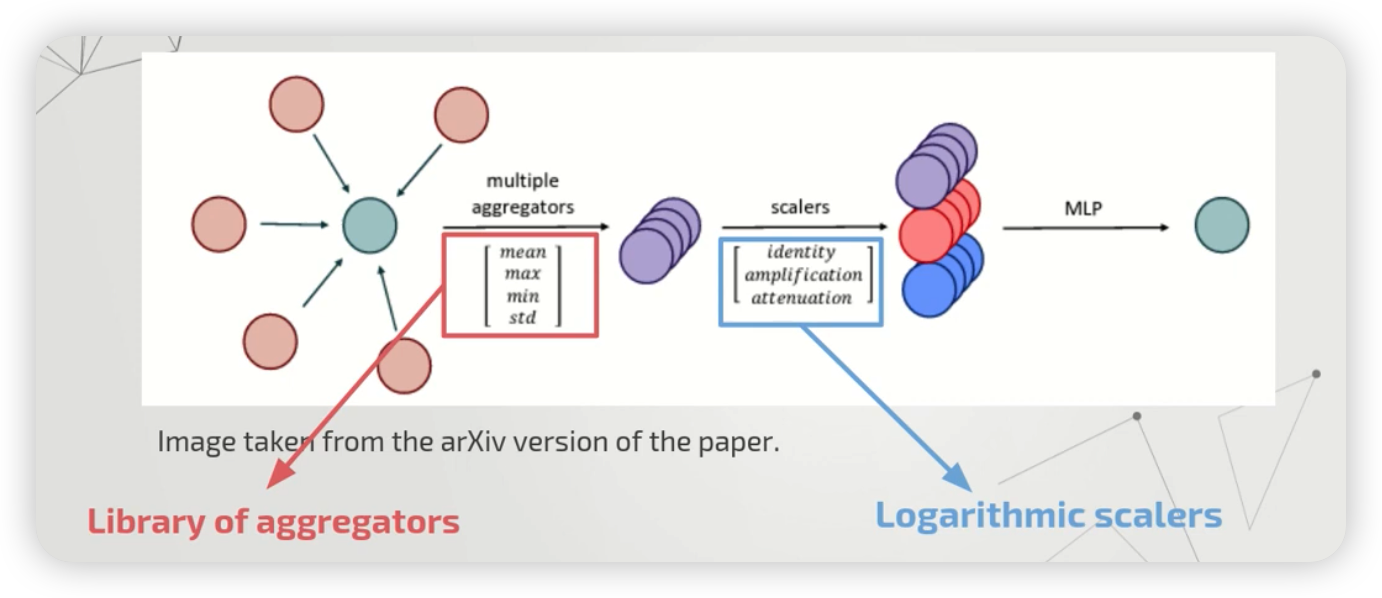
3 종류의 scalers
다양한 종류의 aggregators를 모두 사용해본 뒤, 이들을 scaler들을 사용하여 combine한다.
( \(S_{a m p}, \alpha=1 \quad S_{a t t}, \alpha=-1 \quad S_{\text {identity' }}\) )
- (1) identity
- (2) amplification
- (3) attenuation
\(S=\left(\frac{\log (d+1)}{\delta}\right)^{\alpha}\),
- where \(\delta=\frac{1}{ \mid \operatorname{train} \mid } \sum_{i \in \text { train }} \log \left(d_{i}+1\right)\)
수식 요약
\(\bigoplus=\underbrace{\left[\begin{array}{c} I \\ S(D, \alpha=1) \\ S(D, \alpha=-1) \end{array}\right]}_{\text {scalers }} \otimes \underbrace{\left[\begin{array}{c} \mu \\ \sigma \\ \max \\ \min \end{array}\right]}_{\text {aggregators }}\).
\(X_{i}^{(t+1)}=U\left(X_{i}^{(t)}, \bigoplus_{(j, i) \in E} M\left(X_{i}^{(t)}, E_{j \rightarrow i}, X_{j}^{(t)}\right)\right)\).
4) LAF (Learning Aggregation Functions)
그 밖에도, aggregation function을 학습하는 LAF도 있다.
핵심 : Don’t choose one aggregation function! just learn it
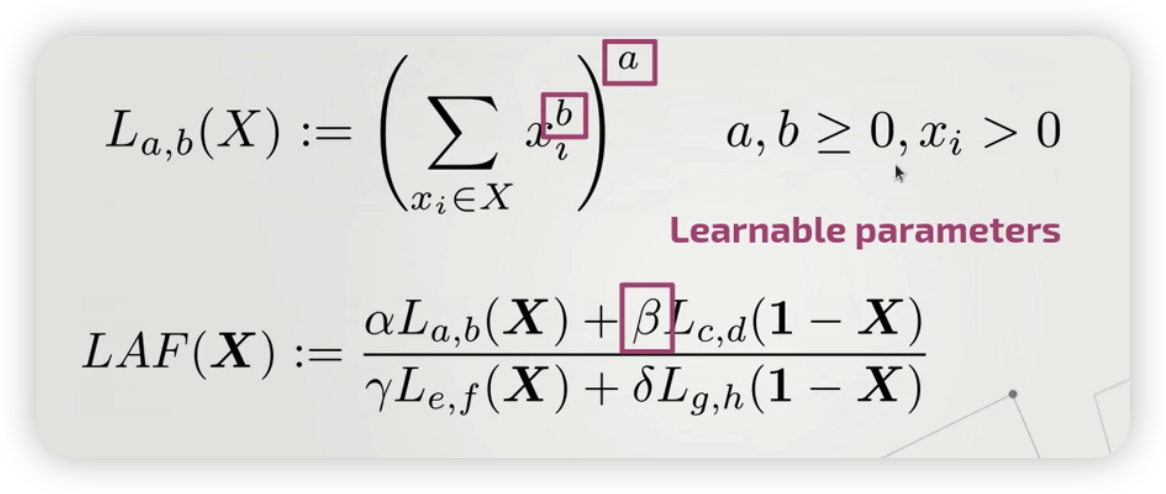
위의 방식으로, 다양한 aggregation function도 나타낼 수 있다.
- ex) MAX, MIN, SUM, MEAN, MOMENTS, COUNT …
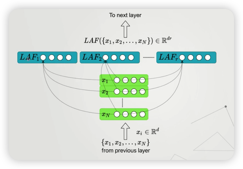
- 위 그림은, 총 \(r\) 개의 LAF를 사용한 뒤 concat한 결과를 나타낸다.
5) Import Packages
import torch
torch.manual_seed(42)
from torch_geometric.nn import MessagePassing
6) Message passing
Message Passing을 위한 2 종류의 대표적인 메소드
- (1)
aggregate( DENSE \(A\) (adjacency matrix)를 사용할 경우 ) - (2)
message_and_aggregate( SPARSE \(A\) (adjacency matrix)를 사용할 경우 )

위 그림을 해석해보자면,
-
같은 색깔 ( = 같은 index로 표현 ) 끼리는, 서로 같은 이웃에 있음을 의미한다.
( 따라서, 같은 색을 가진 input은, 그들 각각의 message가 aggregate되어서 output을 내뱉는다 )
7) LAF aggregation Module
GINConv를 상속 받은 뒤, aggregate 를 overwrite하면 된다.
from torch_geometric.nn import GINConv
from torch.nn import Linear
from laf_model import LAFLayer
class GINLAFConv(GINConv):
    def __init__(self, nn, units=1, node_dim=32, **kwargs):
        super(GINLAFConv, self).__init__(nn, **kwargs)
        # units : 얼마나 많은 LAF를 학습하고 싶은지
        self.laf = LAFLayer(units=units, kernel_initializer='random_uniform')

        # 여러 LAF들의 결과를 concat한 뒤, node_dim으로 매핑시키는 Linear Layer
        self.mlp = torch.nn.Linear(node_dim*units, node_dim)
        self.dim = node_dim
        self.units = units

    def aggregate(self, inputs, index):
        x = torch.sigmoid(inputs)
        x = self.laf(x, index)
        x = x.view((-1, self.dim * self.units))
        x = self.mlp(x)
        return x
8) PNA aggregation module
마찬가지로, GINConv를 상속 받은 뒤, aggregate 를 overwrite하면 된다.
class GINPNAConv(GINConv):
    def __init__(self, nn, node_dim=32, **kwargs):
        super(GINPNAConv, self).__init__(nn, **kwargs)
        self.mlp = torch.nn.Linear(node_dim*12, node_dim)
        self.delta = 2.5749

    def aggregate(self, inputs, index):
        # (1) 4종류의 aggregation function들
        sums = torch_scatter.scatter_add(inputs, index, dim=0)
        maxs = torch_scatter.scatter_max(inputs, index, dim=0)[0]
        means = torch_scatter.scatter_mean(inputs, index, dim=0)
        var = torch.relu(torch_scatter.scatter_mean(inputs ** 2, index, dim=0) - means ** 2)
        aggrs = [sums, maxs, means, var]

        # logarithm of degree 구하기
        c_idx = index.bincount().float().view(-1, 1)
        l_idx = torch.log(c_idx + 1.)

      	# (2) 3종류의 scaler들
        amplification_scaler = [c_idx / self.delta * a for a in aggrs]
        attenuation_scaler = [self.delta / c_idx * a for a in aggrs]

        #
        combinations = torch.cat(aggrs+ amplification_scaler+ attenuation_scaler, dim=1)
        x = self.mlp(combinations)

        return x
9) LAFNet / PNANet
위의 LAF aggregation module을 여러 개 사용하여, 하나의 LAF Net을 만들어보자.
from torch_geometric.nn import MessagePassing, SAGEConv, GINConv, global_add_pool
import torch_scatter
import torch.nn.functional as F
from torch.nn import Sequential, Linear, ReLU
from torch_geometric.datasets import TUDataset
from torch_geometric.data import DataLoader
import os.path as osp
class LAFNet(torch.nn.Module):
    def __init__(self):
        super(LAFNet, self).__init__()

        num_features = dataset.num_features
        dim = 32
        units = 3 # 사용할 LAF의 개수

        nn1 = Sequential(Linear(num_features, dim), ReLU(), Linear(dim, dim))
        nn2 = Sequential(Linear(dim, dim), ReLU(), Linear(dim, dim))
        nn3 = Sequential(Linear(dim, dim), ReLU(), Linear(dim, dim))
        nn4 = Sequential(Linear(dim, dim), ReLU(), Linear(dim, dim))
        nn5 = Sequential(Linear(dim, dim), ReLU(), Linear(dim, dim))

        self.conv1 = GINLAFConv(nn1, units=units, node_dim=num_features)
        self.conv2 = GINLAFConv(nn2, units=units, node_dim=dim)
        self.conv3 = GINLAFConv(nn3, units=units, node_dim=dim)
        self.conv4 = GINLAFConv(nn4, units=units, node_dim=dim)
        self.conv5 = GINLAFConv(nn5, units=units, node_dim=dim)

        self.bn1 = torch.nn.BatchNorm1d(dim)
        self.bn2 = torch.nn.BatchNorm1d(dim)
        self.bn3 = torch.nn.BatchNorm1d(dim)
        self.bn4 = torch.nn.BatchNorm1d(dim)
        self.bn5 = torch.nn.BatchNorm1d(dim)

        self.fc1 = Linear(dim, dim)
        self.fc2 = Linear(dim, dataset.num_classes)

    def forward(self, x, edge_index, batch):
        x = self.bn1(F.relu(self.conv1(x, edge_index)))
        x = self.bn2(F.relu(self.conv2(x, edge_index)))
        x = self.bn3(F.relu(self.conv3(x, edge_index)))
        x = self.bn4(F.relu(self.conv4(x, edge_index)))
        x = self.bn5(F.relu(self.conv5(x, edge_index)))
        x = global_add_pool(x, batch)
        x = F.relu(self.fc1(x))
        x = F.dropout(x, p=0.5, training=self.training)
        x = self.fc2(x)
        return F.log_softmax(x, dim=-1)
-
위 코드에서,
GINLAFConv만GINPNAConv로 바꾸면 PNANet이 된다.GINConv로 바꾸면 GIN이 된다.