
[ 8.Applications of GNNs ]
( 참고 : CS224W: Machine Learning with Graphs )
Contents
- 8-1. Review
- 8-2. Graph Augmentation for GNNs (Intro)
- 8-3. Graph FEATURE Augmentation
- 8-4. Graph STRUCTURE Augmentation
- 8-5. Prediction with GNNs
- 8-6. Training GNNs
- 8-7. Examples
8-1. Review
becareful of adding GNN layers!
\(\rightarrow\) OVER-SMOOTHING problem
then…how to make expressivity with small GNN layers?
- solution 1) Increase the expressive power within each GNN layer
- solution 2) Add layers that do not pass messages
- solution 3) (to use more layers…) use skip-connections
8-2. Graph Augmentation for GNNs (Intro)
raw input graph = computation graph?
\(\rightarrow\) let’s break this assumption!
Reason :
- 1) lack of features
- 2) problems of graph structure
- too sparse \(\rightarrow\) inefficient message passing
- too dense \(\rightarrow\) message passing too costly
- too large \(\rightarrow\) can’t fit graph into a GPU
so…why not use augmentation techniques?
- 1) graph FEATURE augmentation
- to solve “lack of features”
- 2) graph STRUCTURE augmentation
- to solve “problems of graph structure”
- too sparse \(\rightarrow\) add virtual nodes
- too dense \(\rightarrow\) sample neighbors, when message passing
- too large\(\rightarrow\) sample subgraphs
- to solve “problems of graph structure”
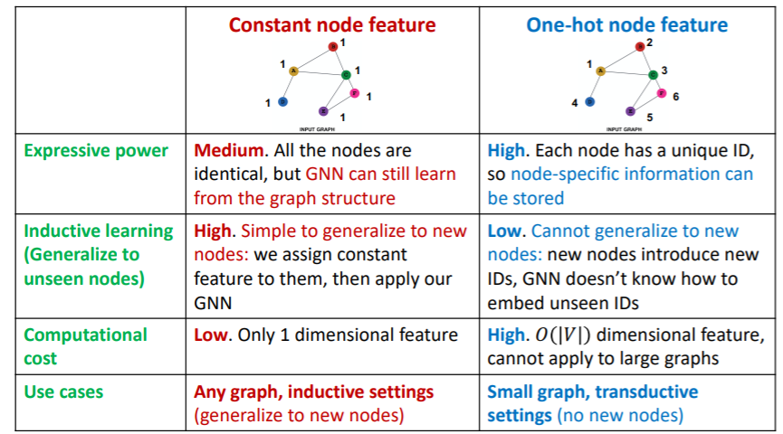
8-3. Graph FEATURE Augmentation
Why?
(1) Reason 1 : input graphs does not have node features
( only have adjacency matrix )
Approach 1 : assign “constant values” to nodes
Approach 2 : assign “unique IDS” to nodes
- convert into one-hot vectors
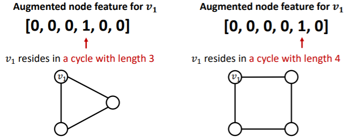
(2) Reason 2 : Certain structures are hard to learn by GNN
example : cycle count feature
- do not know which “length of a cycle” that certain node lives in!
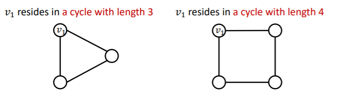
- solution : use cycle count as augmented node features
other augmented features
- node degree
- clustering coefficient
- page rank
- centrality
- ..
8-4. Graph STRUCTURE Augmentation
(1) Virtual Nodes/ Edges
Virtual Edges
- connect 2-hop neighbors via virtual edges
- that is, use \(A+A^2\) for GNN computation
Virtual Nodes
- node that connects to ALL nodes
- all nodes will have distance=2
- benefits : improves message passing ( especially in sparse graphs )
(2) Node Neighborhood Sampling
instead of using all nodes for message passing,
just sample some nodes for message passing !
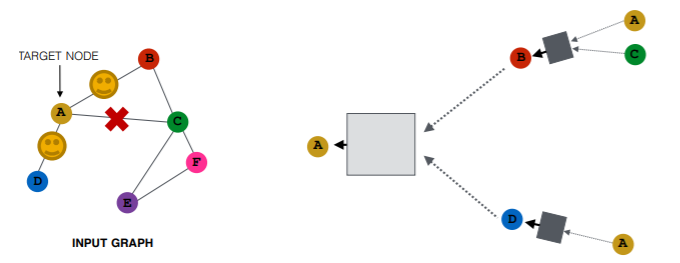
Result
- similar embeddings, when used with ALL nodes
- reduces computational costs
8-5. Prediction with GNNs
(1) Pipeline
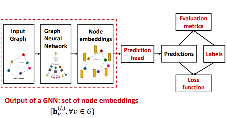
Prediction heads : differ by task levels!
- 1) node-level tasks
- 2) edge-level tasks
- 3) graph-level tasks
(2) Node-level
make prediction (directly) using node embeddings!
- node embeddings : \(\left\{\mathbf{h}_{v}^{(L)} \in \mathbb{R}^{d}, \forall v \in G\right\}\).
- ex) k-way prediction
- classification : \(k\) categories
- regression : \(k\) targets
- prediction : \(\widehat{\boldsymbol{y}}_{v}=\operatorname{Head}_{\text {node }}\left(\mathbf{h}_{v}^{(L)}\right)=\mathbf{W}^{(H)} \mathbf{h}_{v}^{(L)}\)
- \(\mathbf{W}^{(H)} \in \mathbb{R}^{k * d}\).
- \(\mathbf{h}_{v}^{(L)} \in \mathbb{R}^{d}\).
(3) Edge-level
make prediction using pairs of node embeddings
-
ex) k-way prediction
-
prediction : \(\widehat{y}_{u v}=\operatorname{Head}_{\mathrm{edge}}\left(\mathbf{h}_{u}^{(L)}, \mathbf{h}_{v}^{(L)}\right)\)
-
ex 1) concatenation + linear
- \(\left.\widehat{\boldsymbol{y}}_{\boldsymbol{u} v}=\text { Linear(Concat }\left(\mathbf{h}_{u}^{(L)}, \mathbf{h}_{v}^{(L)}\right)\right)\).
- map 2d-dim embeddings to \(k\)-dim embeddings
-
ex 2) dot product
-
\(\widehat{\boldsymbol{y}}_{u v}=\left(\mathbf{h}_{u}^{(L)}\right)^{T} \mathbf{h}_{v}^{(L)}\).
-
only applies to 1-way prediction
( ex. existence of edge )
-
k-way prediction
( like multi-head attention )
- \(\widehat{y}_{u v}^{(1)}=\left(\mathbf{h}_{u}^{(L)}\right)^{T} \mathbf{W}^{(1)} \mathbf{h}_{v}^{(L)}\).
- …
- \(\widehat{y}_{u v}^{(k)}=\left(\mathbf{h}_{u}^{(L)}\right)^{T} \mathbf{W}^{(k)} \mathbf{h}_{v}^{(L)}\).
\(\rightarrow\) \(\widehat{\boldsymbol{y}}_{u v}=\operatorname{Concat}\left(\widehat{y}_{u v}^{(1)}, \ldots, \widehat{y}_{u v}^{(k)}\right) \in \mathbb{R}^{k}\).
-
-
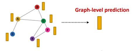
(4) Graph-level
Make prediction using all the node embeddings in our graph
- ex) k-way prediction
- \(\widehat{\boldsymbol{y}}_{G}=\text { Head }_{\text {graph }}\left(\left\{\mathbf{h}_{v}^{(L)} \in \mathbb{R}^{d}, \forall v \in G\right\}\right)\).
Options for prediction head
- global mean pooling : \(\widehat{\boldsymbol{y}}_{G}=\operatorname{Mean}\left(\left\{\mathbf{h}_{v}^{(L)} \in \mathbb{R}^{d}, \forall v \in G\right\}\right)\).
- global max pooling : \(\widehat{\boldsymbol{y}}_{G}=\operatorname{Max}\left(\left\{\mathbf{h}_{v}^{(L)} \in \mathbb{R}^{d}, \forall v \in G\right\}\right)\).
- global sum pooling : \(\widehat{\boldsymbol{y}}_{G}=\operatorname{Sum}\left(\left\{\mathbf{h}_{v}^{(L)} \in \mathbb{R}^{d}, \forall v \in G\right\}\right)\).
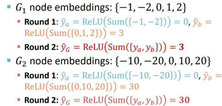
Problems of Global Pooling
-
case : large graph \(\rightarrow\) loss of info
-
ex)
- \(G_1\) : \(\{-1,-2,0,1,2\}\)
- \(G_2\) : \(\{-10,-20,0,10,20\}\)
\(\rightarrow\) should have different embedding,
but in case of global sum pooling, both have 0
Hierarchical Global Pooling
-
Step 1) Separately aggregate \(m\) nodes & last \(n\) nodes
-
Step 2) then, aggregate again to make final prediction
example
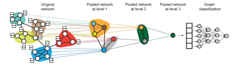
( GNNs at each level can be executed in PARALLEL )
8-6. Training GNNs
what is the ground-truth value?
- case 1) supervised
- comes from external sources
- case 2) unsupverised
- from graph itself
- ( can also say “semi-supervised “)
(1) Supervised Labels
- node labels \(y_v\)
- edge labels \(y_{uv}\)
- graph labels \(y_G\)
all from external sources!
(2) Unsupervised Signals
case when we only have graph, without external labels
- node labels \(y_v\)
- ex) node statistics : clustering coefficients, page rank…
- edge labels \(y_{uv}\)
- ex) link prediction ( hide certain links & predict! )
- graph labels \(y_G\)
- ex) group statistics ( predict if 2 graphs are isomorphic )
\(\rightarrow\) do not require external labels!
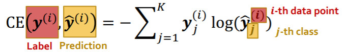
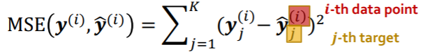
(3) Loss Function
-
Classification : CE loss
-
k-way prediction, for i-th data
-
-
Regression Loss : MSE
-
k-way regression, for i-th data
-
(4) Evaluation
- Regression : RMSE, MAE
- Classification : Accuracy, Precision, Recall, F1-score
(5) Data Split
Random Split
-
randomly split train/val/test set
& average performance over different random seeds
Differ from standard data split!
- reason : data points are NOT INDEPENDENT
- solutions?
Solution 1
-
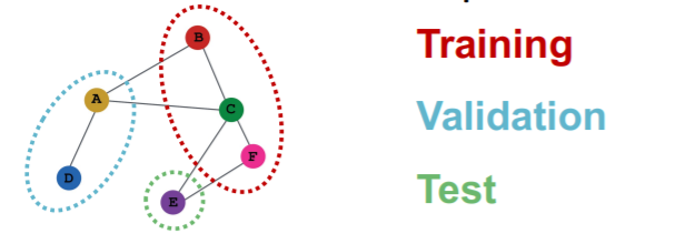
settings : TRANSDUCTIVE
( = input graph can be observed in all the data splits )
-
solution : only split node labels
-
step
- train :
- embedding : ENTIRE graph
- train : node 1&2’s label
- validation :
- embedding : ENTIRE graph
- evaluation : node 3&4’s label
- train :
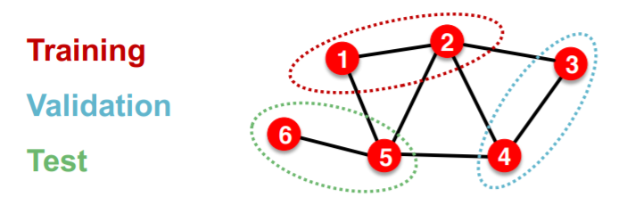
\(\rightarrow\) applicable to node & edge prediction tasks
Solution 2
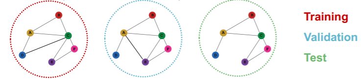
- settings : INDUCTIVE
- solution : break edges between splits \(\rightarrow\) get multiple graphs
- step
- train :
- embedding : node 1&2
- train : node 1&2’s labels
- validation :
- embedding : node 3&4
- evaluation : node 3&4’s labels
- train :
\(\rightarrow\) applicable to node & edge & graph prediction tasks
8-7. Examples
(1) Node Classification
Transductive
-
train/val/test \(\rightarrow\) can observe ENTIRE graph structure,
but observe only their own labels
Inductive
- 3 different graphs ( = all independent )
(2) Graph Classification
Transductive
- impossible
Inductive
- reason : have to test on UNSEEN GRAPHS
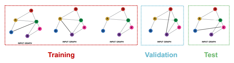
(3) Link Prediction
can be both unsupervised / self-supervised task
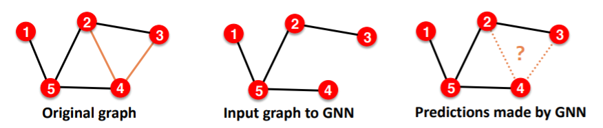
- step 1) hide edges
- step 2) predict edges
Split edges twice
-
step 1) assign 2 types of edges
- (1) MESSAGE edges : for message passing
- (2) SUPERVISION edges : for computing objectives
-
step 2) split train/val/test
-
(option 1) INDUCTIVE link prediction split
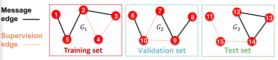
- train : message & supervision edges
- val : message & supervision edges
- test : message & supervision edges
-
(option 2) TRANSDUCTIVE link prediction split
- entire graph is observed in train/val/test split
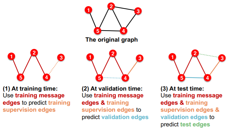
-
need 4 types of edges
- 1) training message edges
- 2) training supervision edges
- 3) validation edges
- 4) test edges
-