Introduction to GNN - Chapter 4) Graph Convolutional Networks

4. Graph Convolutional Networks

GCN : to generalize convolutions to graph domains

4-1. Spectral Methods

SPECTRAL representation of graphs

4 classic models

• (1) Spectral Network
• (2) Chebnet
• (3) GCN
• (4) AGCN

4-1-1. Spectral Network

• convolution operation in Fourier domain

  ( by computing eigendecomposition of graph Laplacian )

• Convolution Operation

  • multiplication of “signal” & “filter”
    • signal : \(\mathbf{x} \in \mathbb{R}^{N}\)
    • filter : \(\mathrm{g}_{\theta}=\operatorname{diag}(\boldsymbol{\theta})\) ( parameterized by \(\mathrm{g}_{\theta}=\operatorname{diag}(\boldsymbol{\theta})\) )
  • \(\mathbf{g}_{\theta} \star \mathbf{x}=\mathbf{U g}_{\theta}(\Lambda) \mathbf{U}^{T} \mathbf{x}\).
    • \(\mathrm{U}\) : matrix of eigenvectors of \(\mathbf{L}\)
      • \(\mathbf{L}=\mathbf{I}_{N}- \mathbf{D}^{-\frac{1}{2}} \mathbf{A} \mathbf{D}^{-\frac{1}{2}}=\mathbf{U} \Lambda \mathbf{U}^{T}\).

• Limitations

  • (1) intense computation
  • (2) non-spatially localized filters

4-1-2. ChebNet

Approximate \(\mathbf{g}_{\theta}(\Lambda)\), by a TRUNCATED expansion,

in terms of Chebyshev polynomials \(\mathbf{T}_{k}(x)\), up to \(K^{th}\) order

( remove the need to compute the eigenvectors of Laplacian )

Spectral Network vs ChebNet

• Spectral Network : \(\mathbf{g}_{\theta} \star \mathbf{x}=\mathbf{U g}_{\theta}(\Lambda) \mathbf{U}^{T} \mathbf{x}\).
• ChebNet : \(\mathbf{g}_{\theta} \star \mathbf{x} \approx \sum_{k=0}^{K} \boldsymbol{\theta}_{k} \mathbf{T}_{k}(\tilde{\mathbf{L}}) \mathbf{x}\)
  • where \(\tilde{\mathbf{L}}=\frac{2}{\lambda_{\max }} \mathbf{L}-\mathbf{I}_{N} \cdot \lambda_{\max }\).
  • \(\mathbf{L} . \theta \in \mathbb{R}^{K}\) : vector of Chebyshev coefficients

Chebyshev Polynomial :

• \(\mathbf{T}_{k}(\mathbf{x})=2 \mathbf{x} \mathbf{T}_{k-1}(\mathbf{x})\),

  where \(\mathbf{T}_{0}(\mathbf{x})=1\) and \(\mathbf{T}_{1}(\mathbf{x})=\mathbf{x}\)

4.1.3. GCN

ChebNet vs GCN

• ChebNet : \(\mathbf{g}_{\theta} \star \mathbf{x} \approx \sum_{k=0}^{K} \boldsymbol{\theta}_{k} \mathbf{T}_{k}(\tilde{\mathbf{L}}) \mathbf{x}\).
• pre-GCN (1) : \(\mathbf{g}_{\theta^{\prime}} \star \mathbf{x} \approx \theta_{0}^{\prime} \mathbf{x}+\theta_{1}^{\prime}\left(\mathbf{L}-\mathbf{I}_{N}\right) \mathbf{x}=\theta_{0}^{\prime} \mathbf{x}-\theta_{1}^{\prime} \mathbf{D}^{-\frac{1}{2}} \mathbf{A} \mathbf{D}^{-\frac{1}{2}} \mathbf{x}\)
  • let \(K=1\) ( to alleviate overfitting on local neighbor )
  • approximate \(\lambda_{\max } \approx 2\)
• pre-GCN (2) : \(\mathbf{g}_{\theta} \star \mathbf{x} \approx \theta\left(\mathbf{I}_{N}+\mathbf{D}^{-\frac{1}{2}} \mathbf{A D}{ }^{-\frac{1}{2}}\right) \mathbf{x} .\)
  • constrain the number of parameters with \(\theta=\theta_{0}^{\prime}=-\theta_{1}^{\prime}\)

Renormalization Trick

• stacking operators above could lead to numerical instabilities
• solution : renormalization trick
  • \(\mathbf{I}_{N}+\) \(\mathbf{D}^{-\frac{1}{2}} \mathbf{A D}{ }^{-\frac{1}{2}} \rightarrow \tilde{\mathbf{D}}^{-\frac{1}{2}} \tilde{\mathbf{A}} \tilde{\mathbf{D}}^{-\frac{1}{2}}\)
    • \(\tilde{\mathbf{A}}=\mathbf{A}+\mathbf{I}_{N}\).
    • \(\tilde{\mathbf{D}}_{i i}=\sum_{j} \tilde{\mathbf{A}}_{i j}\).
  • generalization : \(\mathbf{Z}=\tilde{\mathbf{D}}^{-\frac{1}{2}} \tilde{\mathbf{A}} \tilde{\mathbf{D}}^{-\frac{1}{2}} \mathbf{X} \Theta\)

GCN summary : \(\mathbf{Z}=\tilde{\mathbf{D}}^{-\frac{1}{2}} \tilde{\mathbf{A}} \tilde{\mathbf{D}}^{-\frac{1}{2}} \mathbf{X} \Theta\)

• \(\mathbf{X} \in \mathbb{R}^{N \times C}\) , wth \(C\) channels & \(F\) filters
• \(\Theta \in \mathbb{R}^{C \times F}\) : matrix of filter parameters
• \(\mathbf{Z} \in \mathbb{R}^{N \times F}\) : convolved signal matrix

4-1-4. AGCN

4-1-1 ~ 4-1-3 :

• use the original graph structure

\(\rightarrow\) but….there may be IMPLICIT relation!

\(\rightarrow\) propose ADAPTIVE GCN

Goal : learn underlying relations

• learns “residual” graph laplacian \(\mathbf{L}_{\text {res }}\)

• add it to original laplacian : \(\widehat{\mathbf{L}}=\mathbf{L}+\alpha \mathbf{L}_{\text {res }},\)

Residual graph laplacian : \(\mathbf{L}_{\text {res }}\)

• \(\mathbf{L}_{\text {res }} =\mathbf{I}-\widehat{\mathbf{D}}^{-\frac{1}{2}} \widehat{\mathbf{A}} \widehat{\mathbf{D}}\).
• \(\widehat{\mathbf{D}} =\operatorname{degree}(\widehat{\mathbf{A}})\).
  • \(\widehat{\mathbf{A}}\) : computed with learned metric

learned metric : adaptive to task & input features

• AGCN uses generalized Mahalanobis distance

• \(D\left(\mathbf{x}_{i}, \mathbf{x}_{j}\right)=\sqrt{\left(\mathbf{x}_{i}-\mathbf{x}_{j}\right)^{T} \mathbf{M}\left(\mathbf{x}_{i}-\mathbf{x}_{j}\right)}\),

  where \(\mathbf{M}\) is a learned parameter

  • \(\mathbf{M}=\mathbf{W}_{d} \mathbf{W}_{d}^{T}\),

    where \(\mathbf{W}_d\) is the transform basis to the adaptive space

AGCN

• (1) calculates Gaussian kernel,
  • \(G_{x_{i}, x_{j}}=\exp \left(-D\left(\mathbf{x}_{i}, \mathbf{x}_{j}\right) /\left(2 \sigma^{2}\right)\right)\).
• (2) then normalize G to get \(\hat{\mathbf{A}}\) ( = dense adjacency matrix )

4-2. Spatial Methods

Spectral methods

• learned filters : depend on Laplacian eigenbasis

  ( = depends on graph structure )

• Cons : trained model can not be applied to graph with DIFFERENT structure

Spatial methods

• define convolutions, DIRECTLY on graph
• challenges :
  • (1) defining the convolution operation with differently sized neighborhoods
  • (2) maintaing the local invariance of CNN

4-2-1. Neural FPS

DIFFERENT weight matrixes, for nodes with DIFFERENT degrees

• \(\mathbf{x} =\mathbf{h}_{v}^{t-1}+\sum_{i=1}^{ \mid N_{v} \mid } \mathbf{h}_{i}^{t-1}\).

  • where \(\mathbf{h}_{v}^{t} =\sigma\left(\mathbf{x}\mathbf{W}_{\mathbf{t}}^{ \mid \mathbf{N}_{v} \mid }\right)\)

  • \(\mathbf{W}_{\mathbf{t}}^{ \mid \mathbf{N}_{v} \mid }\) : weight matrix, for nodes with degree \(\mid N_v \mid\)

• adds (1) itself & (2) neighbors

Drawback : can not be applied to LARGE-SCALE graphs ( too large node degree… )

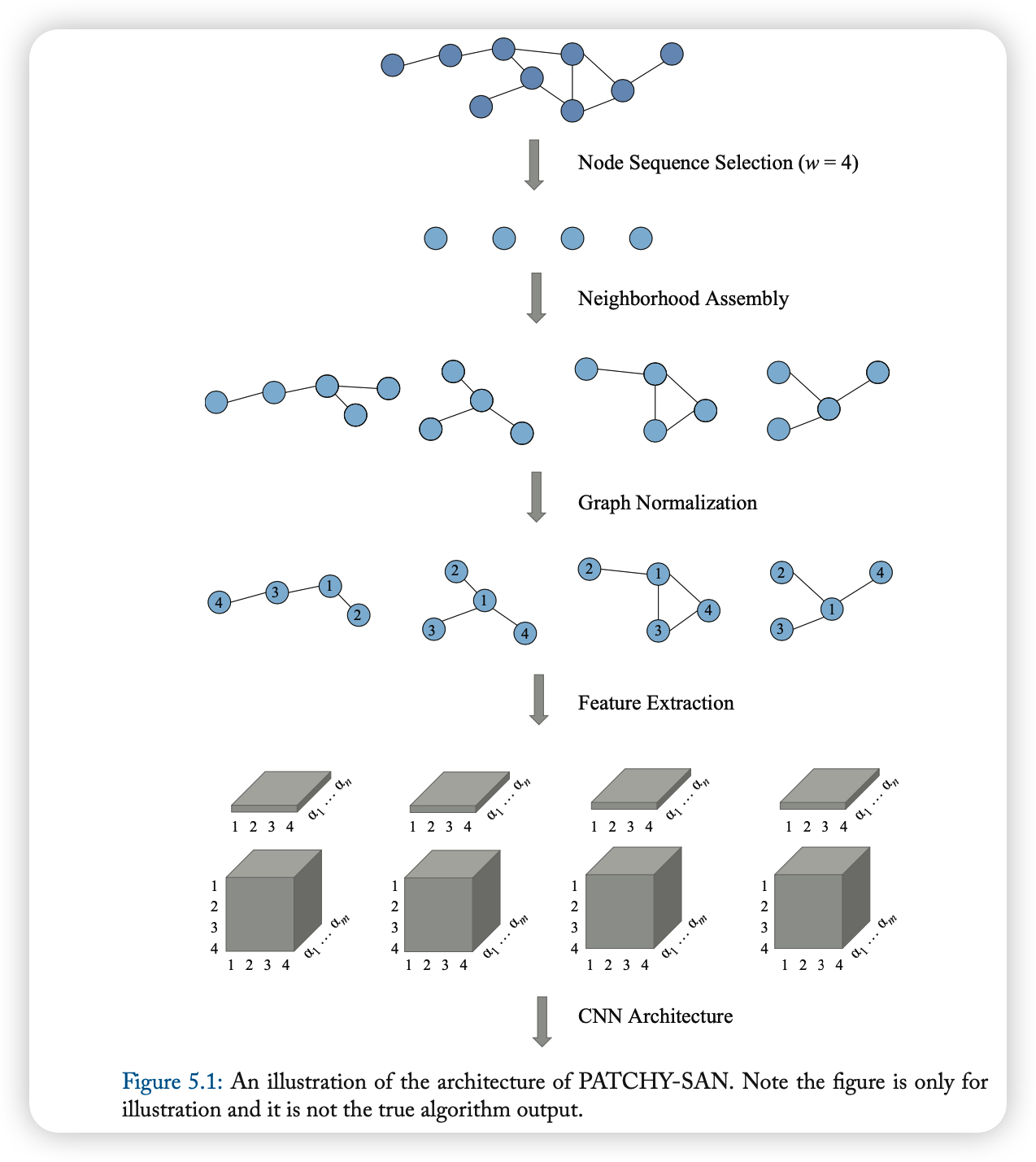
4-2-2. PATCHY-SAN

Simple Steps

• (1) select & normalize \(k\) neighbors ( for each node )
• (2) apply convolution
  • normalized neighborhood = receptive field

Detailed Steps

• (1) Node Sequence Selection
  • do not use all nodes
  • select a sqeuence of nodes
• (2) Neighborhood Asembly
  • BFS, until total of \(k\) neighbors are extracted
• (3) Graph Normalziation
  • Give an order to nodes in receptive field
    • unordered graph -> vector space
  • goal : assign node from 2 different graphs similar relative positions, if they have similar structural roles
• (4) Convolutional Architecture
  • receptive field = normalized neighborhoods
  • channels = node & edge attributes

4-2-3. DCNN

DIFFUSION CNN

• transition matrices are used to define neighbors
• Ex) node classification :
  • \(\mathbf{H}=\sigma\left(\mathbf{W}^{c} \odot \mathbf{P}^{*} \mathbf{X}\right)\).
    • \(\mathbf{X}\) : input features ( shape : \(N \times F\) )
    • \(\mathbf{P}^{*}\) : \(N \times K \times N\) Tensor, which contains power series
      • power series : \(\left\{\mathbf{P}, \mathbf{P}^{2}, \ldots, \mathbf{P}^{K}\right\}\)
    • \(\mathbf{P}\) : degree-normalized transition matrix from adjacency matrix \(\mathbf{A}\)
• result : transformed into diffusion convolutional representation
  • shape ( of each entity ) : \(K \times F\)
    • \(K\) Hops of graph diffusion, over \(F\) features
  • shape ( of full ) : \(N \times K \times F\) ….notation : \(\mathbf{H}\)

For graph classification…

• take average of nodes’ representation
• \(\mathbf{H}=\sigma\left(\mathbf{W}^{c} \odot 1_{N}^{T} \mathbf{P}^{*} \mathbf{X} / N\right)\).

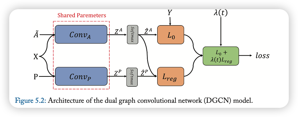
4-2-4. DGCN

Dual GCN … what is dual?

• (1) LOCAL consistency
• (2) GLOBAL consistency

\(\rightarrow\) Uses 2 convolutions ( one supervised loss & one unsupervised loss )

First convolution ( \(C o n v_{A}\) )

• for LOCAL consistency

• original GCN ( \(\mathbf{Z}=\tilde{\mathbf{D}}^{-\frac{1}{2}} \tilde{\mathbf{A}} \tilde{\mathbf{D}}^{-\frac{1}{2}} \mathbf{X} \Theta\) )
• concept : nearby nodes may have similar labels

Second convolution ( \(C o n v_{P}\) )

• for GLOBAL consistency

• replace adjacency matrix, with PPMI matrix

  ( = Positive Pointwise Mutual Information matrix… \(\mathbf{X}_{P}\) )

• \(\mathbf{H}^{\prime}=\sigma\left(\mathbf{D}_{P}^{-\frac{1}{2}} \mathbf{X}_{P} \mathbf{D}_{P}^{-\frac{1}{2}} \mathbf{H} \Theta\right)\).

• concept : nodes with similar context may have similar labels

Ensemble 2 convolutions!

Final Loss function :

• \(L=L_{0}\left(\operatorname{Conv}_{A}\right)+\lambda(t) L_{\text {reg }}\left(\operatorname{Conv}_{A}, \operatorname{Conv}_{P}\right)\).
  • \(L_{0}\left(\operatorname{Conv}_{A}\right)\) : supervised loss ( = CE Loss )
    • \(L_{0}\left(\operatorname{Conv}_{A}\right)=-\frac{1}{ \mid y_{L} \mid } \sum_{l \in y_{L}} \sum_{i=1}^{c} Y_{l, i} \ln \left(\widehat{Z}_{l, i}^{A}\right)\).
  • \(L_{\text {reg }}\left(\operatorname{Conv}_{A}, \operatorname{Conv}_{P}\right)\) : unsupervised loss
    • \(L_{\text {reg }}\left(\operatorname{Conv}_{A}, \operatorname{Conv}_{P}\right)=\frac{1}{n} \sum_{i=1}^{n} \mid \mid \widehat{Z}_{i,:}^{P}-\widehat{Z}_{i,:}^{A} \mid \mid ^{2}\).

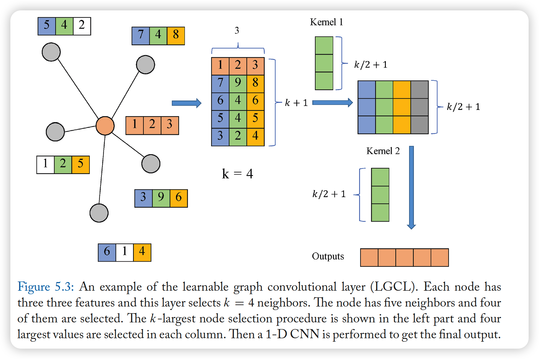
4-2-5. LGCN

Learnable GCN

• based on “LGCL” (Learnable GC Layer) & “sub-graph training strategy”

LGCL (Learnable GCL)

• use CNNs as aggregators

• 2 step

  • (1) get top-k feature elements
  • (2) apply 1-d can

• propagation step :

  • \(\widehat{H}_{t} =g\left(H_{t}, A, k\right)\).
    • \(g\) : k-largest node selection operation
  • \(H_{t+1} =c\left(\widehat{H}_{t}\right)\).
    • \(c\) : regular 1-D CNN

• if less than \(k\)…..then zero-padding

• finally,embedding of node \(x\) is inserted in the first row

  \(\rightarrow\) \(\widehat{M} \in \mathbb{R}^{(k+1) \times c}\)

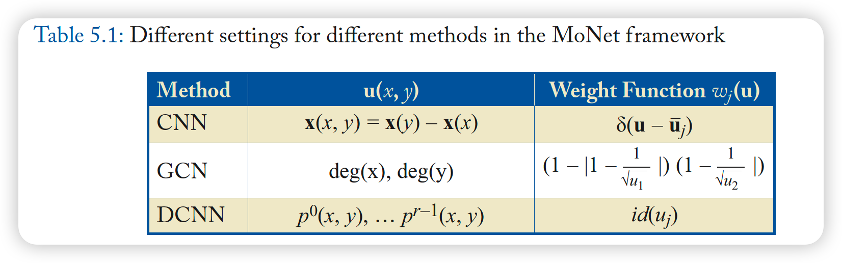
4-2-6. MONET

MoNet ( = spatial domain model ), on non-Euclidean domains

• examples :
  • (1) GCNN ( Geodesic CNN )
  • (2) ACNN ( Anisotropic CNN )
  • (3) GCNN
  • (4) DCNN

MoNet comuptes pseudo-coordinates \(\mathbf{u}(x,y)\)

• use it as weighting function among these coordinates

\(\rightarrow\) \(D_{j}(x) f=\sum_{y \in N_{x}} w_{j}(\mathbf{u}(x, y)) f(y)\).

Then, do convolution, on non-Euclidean domains!

\(\rightarrow\) \((f \star g)(x)=\sum_{j=1}^{J} g_{j} D_{j}(x) f .\)

4-2-7. GraphSAGE

general inductive framework

• generates embeddings, by “sampling” & “aggregating” features

Propagation step :

• \(\mathbf{h}_{N_{v}}^{t} =\text { AGGREGATE }_{t}\left(\left\{\mathbf{h}_{u}^{t-1}, \forall u \in N_{v}\right\}\right)\).
• \(\mathbf{h}_{v}^{t} =\sigma\left(\mathbf{W}^{t} \cdot\left[\mathbf{h}_{v}^{t-1} \mid \mid \mathbf{h}_{N_{v}}^{t}\right]\right)\).

\(\rightarrow\) but, do not use FULL set of neighbors! use UNIFORM SAMPLING

Aggregator functions :

• (1) mean aggregator
• (2) LSTM aggregator
• (3) Pooling aggregator
• ( any symmetric functions can be used )

Also, proposes an UNSUPERVISED loss function

• encourages nearby nodes to have similar representations,

  while distant nodes have different representations

• \(J_{G}\left(\mathbf{z}_{u}\right)=-\log \left(\sigma\left(\mathbf{z}_{u}^{T} \mathbf{z}_{v}\right)\right)-Q \cdot E_{v_{n} \sim P_{n}(v)} \log \left(\sigma\left(-\mathbf{z}_{u}^{T} \mathbf{z}_{v_{n}}\right)\right)\),

  • \(v\) : neighbor of node \(u\)
  • \(P_n\) : negative sampling distribution
  • \(Q\) : number of negative samples