(paper) A3T-GCN ; Attention Temporal GCN for Traffic Forecasting

A3T-GCN : Attention Temporal GCN for Traffic Forecasting (2020)

Contents

1. Abstract
2. A3T-GCN
   1. Definition of Problems
   2. GCN
   3. GRU
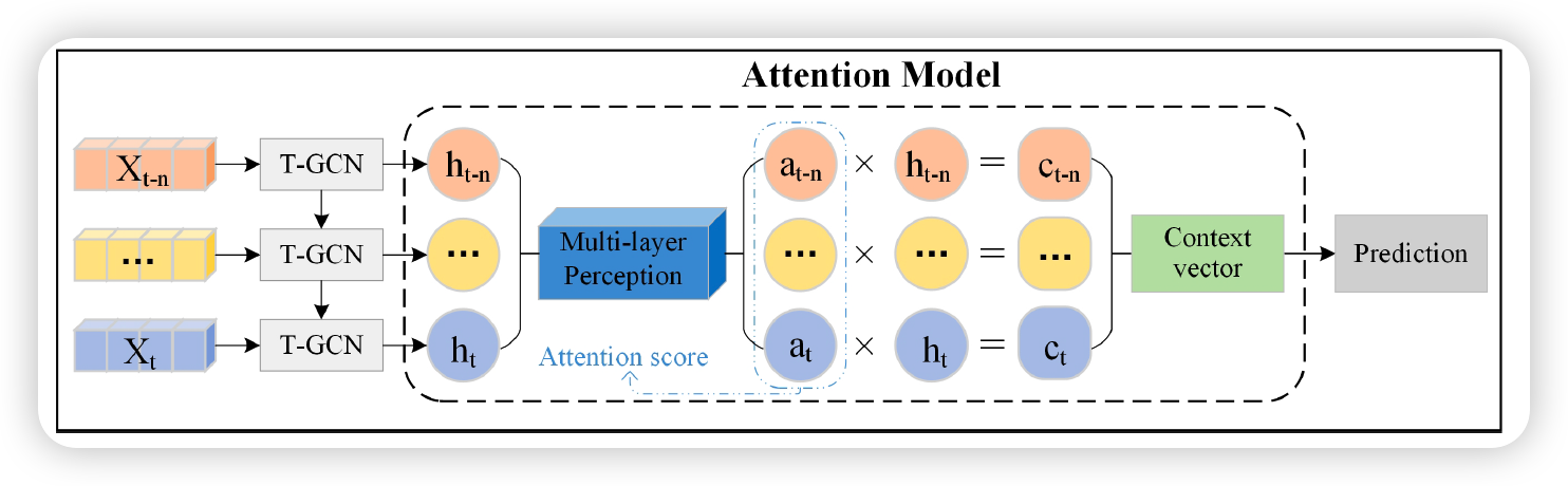
   4. Attention
   5. A3T-GCN
   6. Loss Function

0. Abstract

Traffic Forecasting :

• challenging considering the complex “spatial” and “temporal” dependencies among traffic flows

A3T-GCN (Attention Temporal GCN)

• to simultaneously capture GLOBAL TEMPORAL DYNAMICS & SPATIAL CORRELATIONS
• learns the…
  • (1) short-time trend
    • with GRU
  • (2) spatial dependence
    • based on the topology of road network, with GCN
• use attention ,
  • to adjust the importance of different time points
  • to assemble global temporal information
• source code : https://github.com/lehaifeng/T-GCN/A3T.

1. A3T-GCN

(1) Definition of problems

Notation

• road network : \(G=(V, E)\)
• road section : \(V=\left\{v_{1}, v_{2}, \cdots, v_{N}\right\}\)
• connection between road sections : \(E\)
• adjacency matrix : \(A \in R^{N \times N}\)
• feature matrix : \(X^{N \times P}\)
  • traffic speed on a road section
  • \(P\) : node feature dimension ( = length of historical TS )

Goal :

• predict traffic speeds of future \(T\) moments
• \(\left[X_{t+1}, \cdots, X_{t+T}\right]=f\left(G ;\left(X_{t-n}, \cdots, X_{t-1}, X_{t}\right)\right)\).

(2) GCN

GCN = Semi-supervised models

Spectrum convolution : (1) x (2)

• (1) signal \(x\) on the graph
• (2) figure filter \(g_{\theta}(L)\)
  • constructed in Fourier domain
  • \(g_{\theta}(L) * x=U g_{\theta}\left(U^{T} x\right)\).
  • normalized Laplacian : \(L=I_{N}-D^{-\frac{1}{2}} A D^{-\frac{1}{2}}=U \lambda U^{T}\)
  • graph Fourier transform of \(x\) : \(U^{T} x\)

Multi-layer GCN model : \(H^{(l+1)}=\sigma\left(\widetilde{D}^{-\frac{1}{2}} \widehat{A} \widetilde{D}^{-\frac{1}{2}} H^{(l)} \theta^{(l)}\right)\)

• \(\widetilde{A}=A+I_{N}\),
• \(\widetilde{D}_{i i}=\sum_{j} \widetilde{A}_{i j}\).

ex) 2-layer GCN model : \(f(X, A)=\sigma\left(\widehat{A} \operatorname{ReLU}\left(\widehat{A} X W_{0}\right) W_{1}\right)\)

• \(W_{0} \in R^{P \times H}\) ,
  • where \(P\) = length of time & \(H\) = number of hidden units
• \(W_{1} \in R^{H \times T}\),
  • weight matrix from the hidden layer to the output layer
  • forecast length = \(T\)

(3) GRU

\(\begin{gathered} u_{t}=\sigma\left(W_{u} *\left[X_{t}, h_{t-1}\right]+b_{u}\right) \\ r_{t}=\sigma\left(W_{r} *\left[X_{t}, h_{t-1}\right]+b_{r}\right) \\ c_{t}=\tanh \left(W_{c}\left[X_{t},\left(r_{t} * h_{t-1}\right)\right]+b_{c}\right) \\ h_{t}=u_{t} * h_{t-1}+\left(1-u_{t}\right) * c_{t} \end{gathered}\).

(4) Attention

step 1) \(e_{i}=w_{(2)}\left(w_{(1)} H+b_{(1)}\right)+b_{(2)}\)

step 2) \(\alpha_{i}=\frac{\exp \left(e_{i}\right)}{\sum_{k=1}^{n} \exp \left(e_{k}\right)}\).

step 3) \(C_{t}=\sum_{i=1}^{n} \alpha_{i} * h_{i}\)

• context vector, that covers traffic variation information

(5) A3T-GCN

• improvement of T-GCN ( temporal GCN )

• T-GCN = (1) GCN + (2) GRU

  • [INPUT] backcast length : \(n\)

  • [HIDDEN] \(n\) hidden states

    • \[\left\{h_{t-n}, \cdots, h_{t-1}, h_{t}\right\}\]

      ( = contains “spatio” & “temporal” characteristics )

    • A3T-GCN : put these into attention model

  • [OUTPUT] via FC layer

• T-GCN calculation :

  • \(u_{t}=\sigma\left(W_{u} *\left[G C\left(A, X_{t}\right), h_{t-1}\right]+b_{u}\right)\).
  • \(r_{t}=\sigma\left(W_{r} *\left[G C\left(A, X_{t}\right), h_{t-1}\right]+b_{r}\right)\).
  • \(c_{t}=\tanh \left(W_{c} *\left[G C\left(A, X_{t}\right),\left(r_{t} * h_{t-1}\right)\right]+b_{c}\right)\).
  • \(\left.h_{t}=u_{t} * h_{t-1}+\left(1-u_{t}\right) * c_{t}\right)\).

• Why attention?

  • re-weight the influence of historical traffic states and thus to capture the global variation trends of traffic state

(6) Loss Function

\(\operatorname{loss}=\mid \mid Y_{t}-\widehat{Y}_{t} \mid \mid+\lambda L_{r e g}\).