(paper) ASTGCN ; Attention Based Spatial-Temporal GCN for Traffic Flow Forecasting

ASTGCN : Attention Based Spatial-Temporal GCN for Traffic Flow Forecasting (2019)

Contents

1. Abstract
2. Preliminaries
   1. Traffic Networks
   2. Traffic Flow Forecasting
3. AST-GCN
   1. Spatial Temporal Attention
   2. Spatial Temporal Convolution
   3. Multi-component Fusion

0. Abstract

Existing methods

• lacking abilities of modeling the dynamic spatial-temporal correlations of traffic data

ASTGCN

• Attention based spatial-temporal GCN

• consists of 3 independent components,

  to model 3 temporal properties

  • (1) recent
  • (2) daily-periodic
  • (3) weekly-periodic

• each component contains 2 major parts

  • (a) spatial-temporal attention

    \(\rightarrow\) to capture the dynamic spatial temporal correlation

  • (b-1) spatial-temporal convolution

    \(\rightarrow\) to capture the spatial patterns

  • (b-2) common standard convolutions

    \(\rightarrow\) to capture the temporal patterns

output of 3 components are fused \(\rightarrow\) final result!

1. Preliminaries

(1) Traffic Networks

\(N\) nodes = \(N\) devices

• each device has \(F\) measurements ( = \(F\)-dim feature vector )

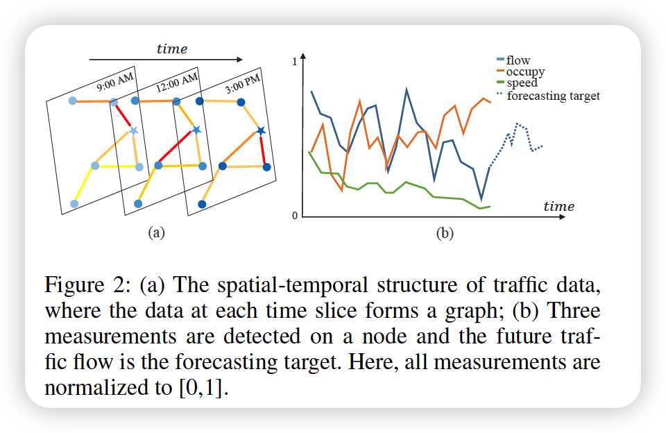
(2) Traffic Flow Forecasting

Notation

• \(f\)-th time series on each node ( \(f \in\) \((1, \ldots, F))\)
• \(\mathcal{X}=\left(\mathbf{X}_{1}, \mathbf{X}_{2}, \ldots, \mathbf{X}_{\tau}\right)^{T} \in \mathbb{R}^{N \times F \times \tau}\).
  • \(\mathbf{x}_{t}^{i} \in \mathbb{R}^{F}\) : values of ALL features of node \(i\) at time \(t\)
    • \(x_{t}^{c, i} \in \mathbb{R}\) : \(c\)-th feature of node \(i\) at time \(t\)
• \(y_{t}^{i}=x_{t}^{f, i} \in \mathbb{R}\) : traffic flow of node \(i\) at time \(t\) in the future

Problem

• given \(\mathcal{X}\), ( window size = \(\tau\) )
• predict \(\mathbf{Y}=\left(\mathbf{y}^{1}, \mathbf{y}^{2}, \ldots, \mathbf{y}^{N}\right)^{T} \in \mathbb{R}^{N \times T_{p}}\)

2. AST-GCN

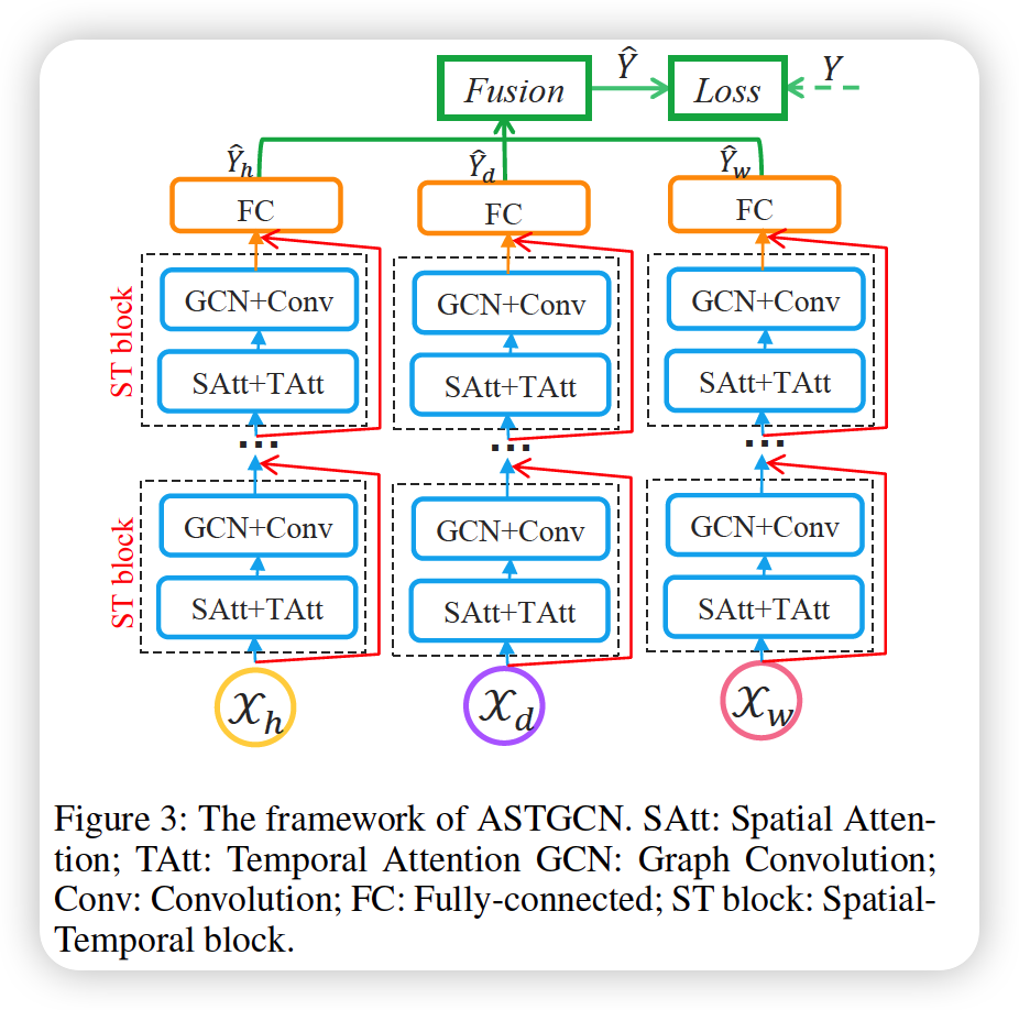
• 3 independent components
  • \(h\) : recent
  • \(d\) : daily-periodic
  • \(w\) : weekly-periodic

Notation

• sampling frequency : \(q\) times per day
• current time : \(t_0\)
• forecast horizon : \(T_p\)
• \(T_h, T_d, T_w\) : length of 3 TS segments
  • all interger multiples of \(T_p\)

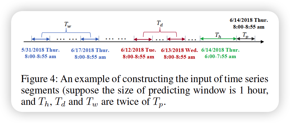
RECENT segment

\(\mathcal{X}_{h}=\left(\mathbf{X}_{t_{0}-T_{h}+1}, \mathbf{X}_{t_{0}-T_{h}+2}, \ldots, \mathbf{X}_{t_{0}}\right) \in \mathbb{R}^{N \times F \times T_{h}}\).

DAILY-PERIODIC segment

\(\begin{aligned} &\mathcal{X}_{d}=\left(\mathbf{X}_{t_{0}-\left(T_{d} / T_{p}\right) * q+1}, \ldots, \mathbf{X}_{t_{0}-\left(T_{d} / T_{p}\right) * q+T_{p}},\right. \\ &\mathbf{X}_{t_{0}-\left(T_{d} / T_{p}-1\right) * q+1}, \ldots, \mathbf{X}_{t_{0}-\left(T_{d} / T_{p}-1\right) * q+T_{p}}, \ldots \end{aligned}\).

WEEKLY-PERIODIC segment

\[\mathcal{X}_{w}=\left(\mathbf{X}_{t_{0}-7 *\left(T_{w} / T_{p}\right) * q+1}, \ldots, \mathbf{X}_{t_{0}-7 *\left(T_{w} / T_{p}\right) * q+T_{p}}\right. \text {, }\]

\(\begin{aligned} &\mathbf{X}_{t_{0}-7 *\left(T_{w} / T_{p}-1\right) * q+1}, \ldots, \mathbf{X}_{t_{0}-7 *\left(T_{w} / T_{p}-1\right) * q+T_{p}}, \ldots \\ &\left.\mathbf{X}_{t_{0}-7 * q+1}, \ldots, \mathbf{X}_{t_{0}-7 * q+T_{p}}\right) \in \mathbb{R}^{F \times N \times T_{w}} \end{aligned}\).

Summary

• 3 components share same structure
• each structure consists of several spatial-temporal blocks & FC layer
• spatial-temporal blocks
  • (1) spatial-temporal attention module
  • (2) spatial-temporal convolution module
• adopt a residual learning framework
• output of 3 components are merged!

(1) Spatial Temporal Attention

2 kinds of attention

• (1) spatial attention
• (2) temporal attention

a) spatial attention

ex) recent component

\(\mathbf{S}=\mathbf{V}_{s} \cdot \sigma\left(\left(\mathcal{X}_{h}^{(r-1)} \mathbf{W}_{1}\right) \mathbf{W}_{2}\left(\mathbf{W}_{3} \mathcal{X}_{h}^{(r-1)}\right)^{T}+\mathbf{b}_{s}\right)\),

• \(\mathbf{S}_{i, j}^{\prime}=\frac{\exp \left(\mathbf{S}_{\mathrm{i}, \mathrm{j}}\right)}{\sum_{j=1}^{N} \exp \left(\mathbf{S}_{\mathrm{i}, \mathrm{j}}\right)}\),

• \(\mathcal{X}_{h}^{(r-1)}=\left(\mathbf{X}_{1}, \mathbf{X}_{2}, \ldots \mathbf{X}_{T_{r-1}}\right) \in \mathbb{R}^{N \times C_{r-1} \times T_{r-1}}\),

  • input of the \(r^{t h}\) spatial-temporal block

  • when \(r=1, C_{0}=F\)

  • \(T_{r-1}\) : length of temporal dimension in \(r^{th}\) layer

attention matrix \(\mathbf{S}\) is dynamically computed

( according to the current input )

• \(\mathbf{S}_{i,j}\) : correlation strength between node \(i\) & \(j\)

when performing GCN, use 2 matrix

• (1) adjacency matrix : \(\mathbf{A}\)
• (2) spatial attention matrix : \(\mathbf{S}^{\prime} \in \mathbb{R}^{N \times N}\)

b) temporal attention

\(\mathbf{E}=\mathbf{V}_{e} \cdot \sigma\left(\left(\left(\boldsymbol{\mathcal { X }}_{h}^{(r-1)}\right)^{T} \mathbf{U}_{1}\right) \mathbf{U}_{2}\left(\mathbf{U}_{3} \mathcal{X}_{h}^{(r-1)}\right)+\mathbf{b}_{e}\right)\).

• \(\mathbf{E}_{i, j}^{\prime}=\frac{\exp \left(\mathbf{E}_{\mathrm{i}, \mathrm{j}}\right)}{\sum_{j=1}^{T_{r-1}} \exp \left(\mathbf{E}_{\mathrm{i}, \mathrm{j}}\right)}\).
  • temporal correlation matrix \(\mathbf{E}\) is determined by the varying inputs
  • correlation strength between time \(i\) & \(j\)

Adjusted Input

\[\hat{\mathcal{X}}_{h}^{(r-1)}=\left(\hat{\mathbf{X}}_{1}, \hat{\mathbf{X}}_{2}, \ldots, \hat{\mathbf{X}}_{T_{r-1}}\right)=\left(\mathbf{X}_{1}, \mathbf{X}_{2}, \ldots, \mathbf{X}_{T_{r-1}}\right) \mathbf{E}^{\prime} \in \mathbb{R}^{N \times C_{r-1} \times T_{r-1}}\]

(2) spatial-temporal convolution

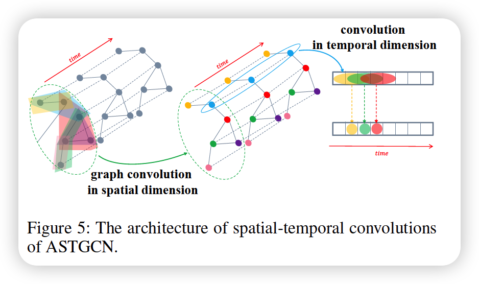
a) Graph convolution in spatial dimension

\(g_{\theta} *_{G} x=g_{\theta}(\mathbf{L}) x=\sum_{k=0}^{K-1} \theta_{k} T_{k}(\tilde{\mathbf{L}}) x\).

• \(\theta \in \mathbb{R}^{K}\).
• \(\tilde{\mathbf{L}}=\frac{2}{\lambda_{\max }} \mathbf{L}-\mathbf{I}_{N}\).
• \(T_{k}(x)=2 x T_{k-1}(x)-T_{k-2}(x)\).

In order to dynamically adjust the correlations between nodes,

for each term of Chebyshev polynomial, use \(T_{k}(\widetilde{\mathbf{L}})\) with \(\mathbf{S}^{\prime} \in \mathbb{R}^{N \times N}\)

\(\rightarrow\) \(g_{\theta} *_{G} x=g_{\theta}(\mathbf{L}) x=\sum_{k=0}^{K-1} \theta_{k}\left(T_{k}(\tilde{\mathbf{L}}) \odot \mathbf{S}^{\prime}\right) x\)

Generalize this! can see it as mutiple channels

• input : \(\hat{\mathcal{X}}_{h}^{(r-1)}=\left(\hat{\mathbf{X}}_{1}, \hat{\mathbf{X}}_{2}, \ldots, \hat{\mathbf{X}}_{T_{r-1}}\right) \in \mathbb{R}^{N \times C_{r-1} \times T_{r-1}}\)

  • feature of node have \(C_{r-1}\) channels

  • for each time step \(t\), perform \(C_{r}\) filters on the graph \(\hat{\mathbf{X}}_{t}\)

    ( kernel : \(\Theta=\left(\Theta_{1}, \Theta_{2}, \ldots, \Theta_{C_{r}}\right) \in \mathbb{R}^{K \times C_{r-1} \times C_{r}}\) )

    \(\rightarrow\) get \(g_{\theta} *_{G} \hat{\mathbf{X}}_{t}\)

b) Convolution in temporal dimension

\(\mathcal{X}_{h}^{(r)}=\operatorname{ReLU}\left(\Phi *\left(\operatorname{ReLU}\left(g_{\theta} *_{G} \hat{\mathcal{X}}_{h}^{(r-1)}\right)\right)\right) \in \mathbb{R}^{C_{r} \times N \times T_{r}}\).

(3) Multi-Component Fusion

\(\hat{\mathbf{Y}}=\mathbf{W}_{h} \odot \hat{\mathbf{Y}}_{h}+\mathbf{W}_{d} \odot \hat{\mathbf{Y}}_{d}+\mathbf{W}_{w} \odot \hat{\mathbf{Y}}_{w}\).