(paper) GMAN ; A Graph Multi-Attention Network for Traffic Prediction

GMAN : A Graph Multi-Attention Network for Traffic Prediction (2019)

Contents

1. Abstract
2. Preliminaries
3. GMAN ( Graph Multi-Attention Network )
   1. Spatio-Temporal Embedding
   2. ST-Attention Block
      1. spatial attention
      2. temporal attention
      3. gated fusion
      4. transform attention
      5. encoder-decoder

0. Abstract

goal : long-term traffic prediction

this paper

• focus on spatio-temporal factors
• propose GMAN (Graph Multi-attention Network)

GMAN

• (1) encoder-decoder

  • both consists of multiple spatio-temporal attention block

• (2) between encoder & decoder

  • transform attention layer

    = models the direct relationshipbs between past & future time steps

    = help alleviate error propagation problem

code : https://github.com/zhengchuanpan/GMAN

1. Preliminaries

Road network ( WEIGHTED & DIRECTED graph ) : \(\mathcal{G}=(\mathcal{V}, \mathcal{E}, \mathcal{A})\)

• \(\mathcal{V}\) : traffic sensors ( \(N=\mid \mathcal{V} \mid\) )
• \(\mathcal{E}\) : edges
• \(\mathcal{A} \in \mathbb{R}^{N \times N}\) : weighted adjacency matrix
  • \(\mathcal{A}_{v_{i}, v_{j}}\) : proximity (measured by the road network distance)
• \(X_{t} \in \mathbb{R}^{N \times C}\) : traffic condition at time \(t\)
  • \(C\) : # of traffic conditions (e.g., traffic volume, traffic speed, etc.)

Goal :

• (input) : \(\mathcal{X}=\left(X_{t_{1}}, X_{t_{2}}, \ldots, X_{t_{P}}\right) \in \mathbb{R}^{P \times N \times C}\)
• (prediction) : \(\hat{Y}=\left(\hat{X}_{t+1}, \hat{X}_{t_{P+2}}, \ldots, \hat{X}_{t_{P+Q}}\right) \in \mathbb{R}^{Q \times N \times C}\)

2. GMAN ( Graph Multi-Attention Network )

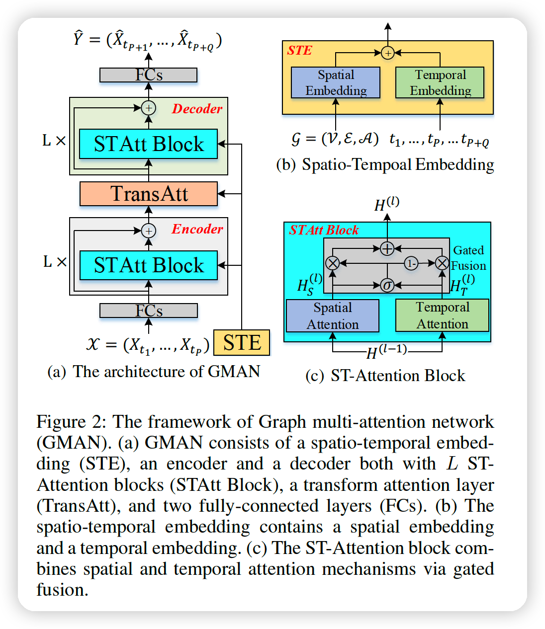
Encoder & Decoder

• encoder : \(L\) ST-attention blocks + residual connection
• decoder : \(L\) ST-attention blocks + residual connection

ST-attention block

• composed of spatial & temporal attention, with gated fusion

Transform Attention layer

• between encoder & decoder
• convert the encoded features to the decoder

etc

• incoroprate the “graph structure” & “time info” into multi-head attention through a spatio-temporal embedding (STE)
• to facilitate residual connection, all layers produce D-dim output

(1) Spatio-Temporal Embedding

a) Spatial embedding

• leverage the node2vec approach to learn the node representations

• to co-train the pre-learned vectors with the whole model,

  these vectors are fed into a 2 FC layers

  \(\rightarrow\) obtain the spatial embedding ( \(e_{v_{i}}^{S} \in \mathbb{R}^{D}\) )

• BUT … only provides static representations ( dynamic correlations X )

b) Temporal Embedding

• to encode each time step into a vector

• encode the day-of-week and time-of-day of each time step,

  into \(\mathbb{R}^{7}\) and \(\mathbb{R}^{T}\) , using one-hot coding & concatenate them into \(\mathbb{R}^{T+7}\)

• Also fed into a 2 FC layers, and get \(D\) Dim vector

• embed time features for both “historical \(P\)” & “future \(Q\)” time-steps

  • (1) \(e_{t_{j}}^{T} \in \mathbb{R}^{D}\) , where \(t_{j}=t_{1}, \ldots, t_{P}, \ldots, t_{P+Q}\)

c) spatio-temporal embedding (STE)

Goal : fuse Spatial & Temporal embedding

STE : \(e_{v_{i}, t_{j}}=e_{v_{i}}^{S}+e_{t_{j}}^{T}\) ….. for vertex \(v_{i}\) at time step \(t_{j}\)

\(\rightarrow\) STE of \(N\) vertices, in \(P+Q\) time steps : \(E \in\mathbb{R}^{(P+Q) \times N \times D}\)

contains both (1) graph structure and (2) time information

\(\rightarrow\) will be used in spatial, temporal and transform attention mechanisms.

(2) ST-Attention Block

includes 3 things

• (1) spatial attention
• (2) temporal attention
• (3) gated fusion

Notation

• INPUT of \(l^{th}\) block : \(H^{(l-1)}\)
  • \(h_{v_{i}, t_{j}}^{(l-1)}\) : hidden state of \(v_{i}\) at time step \(t_{j}\)
• OUTPUT of 2 attentions : \(H_{S}^{(l)}\) & \(H_{T}^{(l)}\)
  • \(H_{S}^{(l)}\) : spatial ~
    • \(h s_{v_{i}, t_{j}}^{(l)}\) : hidden state of ~
  • \(H_{T}^{(l)}\) : temporal ~
    • \(h t_{v_{i}, t_{j}}^{(l)}\) : hidden state of ~
• OUTPUT of \(l^{th}\) block ( after gated fusion ) : \(H^{(l)}\)

Affine (non-linear) transformation :

• \(f(x)=\operatorname{ReLU}(x \mathbf{W}+\mathbf{b})\).

Spatial attention

Correlation : highly dynamic, changing over time

\(\rightarrow\) use spatial attention , to adaptively capture the correlations between sensors

Key idea : dynamically assign different weights to different nodes

Attention Result :

• \(h s_{v_{i}, t_{j}}^{(l)}=\sum_{v \in \mathcal{V}} \alpha_{v_{i}, v} \cdot h_{v, t_{j}}^{(l-1)}\).

both the current traffic conditions and the road network structure

\(\rightarrow\) could affect the correlations between sensors

\(\rightarrow\) thus, consider both Traffic features & graph structure

( concatenate the hidden state with the spatio-temporal embedding )

to compute the relevance between vertex \(v_{i}\) and \(v\) :

• \(s_{v_{i}, v}=\frac{\left\langle h_{v_{i}, t_{j}}^{(l-1)} e_{v_{i}, t_{j}}, h_{v, t_{j}}^{(l-1)} \mid \mid e_{v, t_{j}}\right\rangle}{\sqrt{2 D}}\).

use Multi(=\(K\)) head attention

use group spatial attention

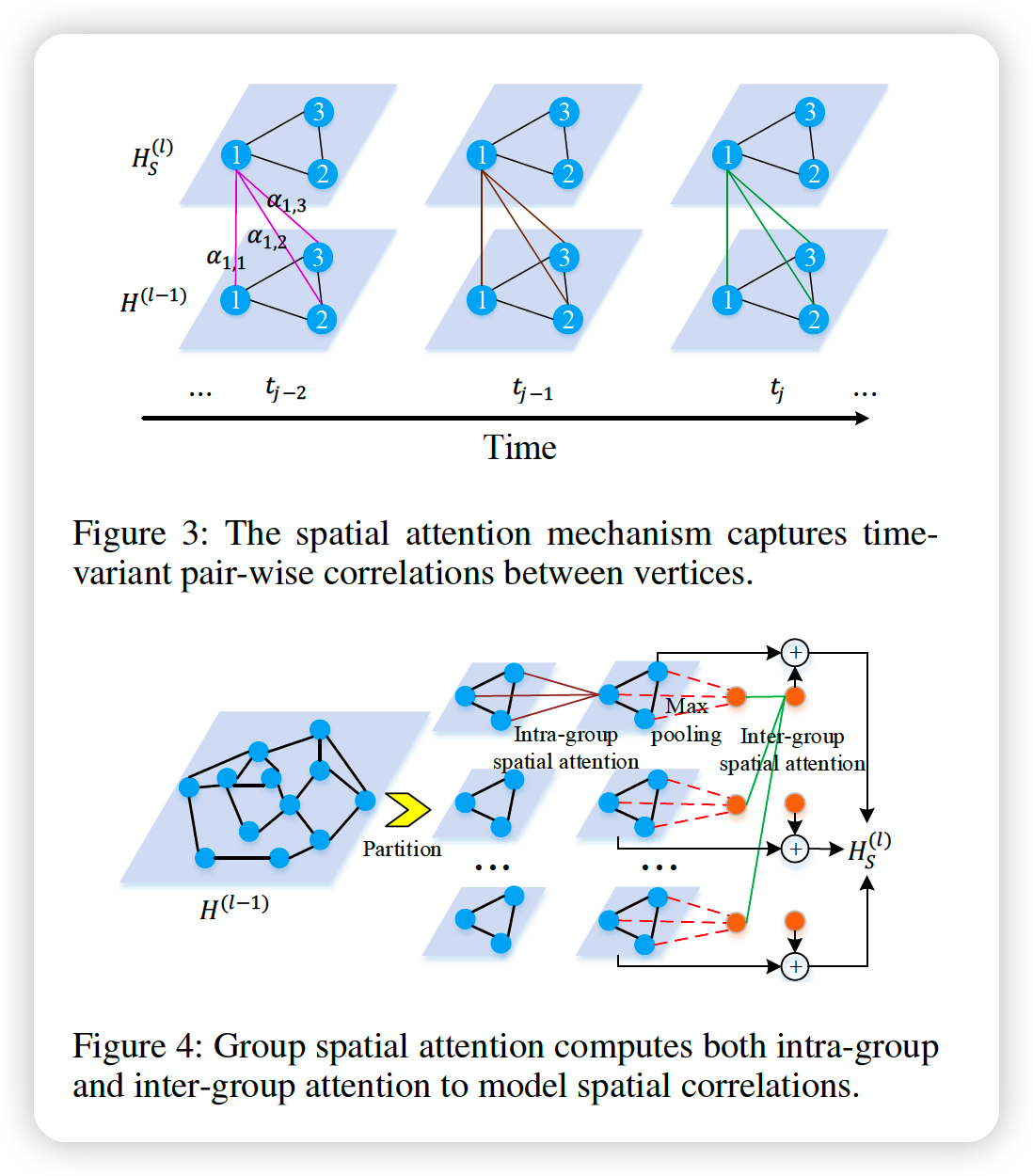
partition \(N\) nodes into \(G\) groups

• each group : \(M = N/G\) nodes

• in each group, we compute intra-group attention

• then, apply max-pooling in each group to get one representation

• then, compute the inter-group attention to model correlations between groups

  \(\rightarrow\) produce a global feature for each group

• then, local feature is added to it \(\rightarrow\) final output!

Temporal attention

to adaptively model the non-linear correlations between different time steps

temporal correlation

• influenced by both (1) traffic condition & (2) time context

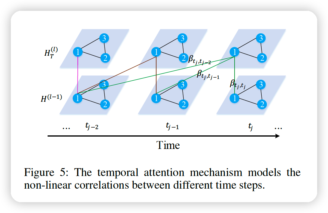
Correlation between \(t_j\) & \(t\) :

\[\begin{gathered} u_{t_{j}, t}^{(k)}=\frac{\left\langle f_{t, 1}^{(k)}\left(h_{v_{i}, t_{j}}^{(l-1)} \mid \mid e_{v_{i}, t_{j}}\right), f_{t, 2}^{(k)}\left(h_{v_{i}, t}^{(l-1)} \mid \mid e_{v_{i}, t}\right)\right\rangle}{\sqrt{d}} \\ \beta_{t_{j}, t}^{(k)}=\frac{\exp \left(u_{t_{j}, t}^{(k)}\right)}{\sum_{t_{r} \in \mathcal{N}_{t_{j}}} \exp \left(u_{t_{j}, t_{r}}^{(k)}\right)} \end{gathered}\]

• \(\beta_{t_{j}, t}^{(k)}\) : attention score in \(k^{th}\) head

\(h t_{v_{i}, t_{j}}^{(l)}= \mid \mid _{k=1}^{K}\left\{\sum_{t \in \mathcal{N}_{t_{j}}} \beta_{t_{j}, t}^{(k)} \cdot f_{t, 3}^{(k)}\left(h_{v_{i}, t}^{(l-1)}\right)\right\}\).

Gated fusion

to adaptively fuse the spatial and temporal representations

Input : output of attentions

• \(H_{S}^{(l)}\) and \(H_{T}^{(l)}\)
  • shape : (encoder) \(\mathbb{R}^{P \times N \times D}\)
  • shape : (decoder) \(\mathbb{R}^{Q \times N \times D}\)

Fusion : \(H^{(l)}=z \odot H_{S}^{(l)}+(1-z) \odot H_{T}^{(l)}\),

• where \(z=\sigma\left(H_{S}^{(l)} \mathbf{W}_{z, 1}+H_{T}^{(l)} \mathbf{W}_{z, 2}+\mathbf{b}_{z}\right)\)
  • where \(\mathbf{W}_{z, 1} \in \mathbb{R}^{D \times D}, \mathbf{W}_{z, 2} \in \mathbb{R}^{D \times D}\) and \(\mathbf{b}_{z} \in \mathbb{R}^{D}\)

Transform attention

• to ease the error propagation effect

• models the direct relationship between each future time step and every historical time step to convert the encoded traffic features to generate future representations as the input of the decoder.

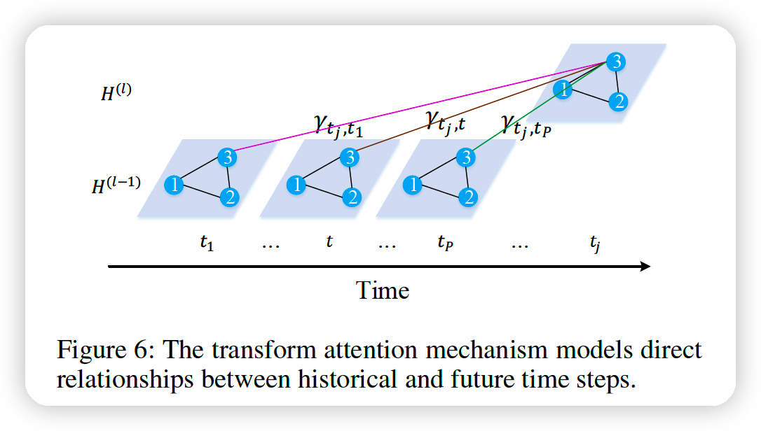
for vertex \(v_{i}\), the relevance between the prediction time step \(t_{j}\left(t_{j}=t_{P+1}, \ldots, t_{P+Q}\right)\) and the historical time step \(t\left(t=t_{1}, \ldots, t_{P}\right)\) :

\(\rightarrow\) measured by spatio-temporal embedding:

\(\lambda_{t_{j}, t}^{(k)}=\frac{\left\langle f_{t r, 1}^{(k)}\left(e_{v_{i}, t_{j}}\right), f_{t r, 2}^{(k)}\left(e_{v_{i}, t}\right)\right\rangle}{\sqrt{d}}\).

\(\gamma_{t_{j}, t}^{(k)}=\frac{\exp \left(\lambda_{t_{j}, t}^{(k)}\right)}{\sum_{t_{r}=t_{1}}^{t_{P}} \exp \left(\lambda_{t_{j}, t_{r}}^{(k)}\right)}\).

\(\rightarrow\) \(h_{v_{i}, t_{j}}^{(l)}= \mid \mid _{k=1}^{K}\left\{\sum_{t=t_{1}}^{t_{P}} \gamma_{t_{j}, t}^{(k)} \cdot f_{t r, 3}^{(k)}\left(h_{v_{i}, t}^{(l-1)}\right)\right\}\)

Encoder-decoder

Summary

• step 1) historical observation \(\mathcal{X} \in \mathbb{R}^{P \times N \times C}\) is transformed to \(H^{(0)} \in\) \(\mathbb{R}^{P \times N \times D}\) using fully-connected layers.
• step 2) \(H^{(0)}\) is fed into the encoder with \(L\) ST-Attention blocks
  • produces an output \(H^{(L)} \in \mathbb{R}^{P \times N \times D}\)
• step 3) transform attention layer is added
  • convert the encoded feature \(H^{(L)}\) to generate the future sequence representation \(H^{(L+1)} \in \mathbb{R}^{Q \times N \times D}\)
• step 4) decoder stacks \(L \mathrm{ST}\) Attention blocks upon \(H^{(L+1)}\), and produces the output as \(H^{(2 L+1)} \in \mathbb{R}^{Q \times N \times D}\)
• step 5) fully-connected layers produce the \(Q\) time steps ahead prediction \(\hat{Y} \in \mathbb{R}^{Q \times N \times C}\).

Loss Function : \(\mathcal{L}(\Theta)=\frac{1}{Q} \sum_{t=t_{P+1}}^{t_{P+Q}} \mid Y_{t}-\hat{Y}_{t} \mid\)