(paper) Graph Attention Networks

Graph Attention Networks (2017, 2820)

Contents

1. Abstract
2. Introduction
3. GAT architecture
   1. Graph Attentional Layer

0. Abstract

GAT (Graph Attention Networks)

• leveraging masked self-attentional layers
• address the shortcomings of prior methods based on graph convolutions
• stack layers, in which nodes are able to attend over their neighborhoods’ features
• enable (implicitly) specifying different weights to different nodes in a neighborhood,
  • without requiring any kind of costly matrix operation
  • without depending on knowing the graph structure

1. Introduction

• introduce an attention-based architecture to perform node classification of graph-structured data.
• Key idea :
  • compute the hidden representations of each node, by attending over its neighbors, following a self-attention strategy
  • attention
    • (1) parallelizable
    • (2) can be applied to graph nodes having different degrees by specifying arbitrary weights to the neighbors
    • (3) directly applicable to inductive learning problems

2. GAT architecture

building block layer

• used to construct arbitrary graph attention network

(1) Graph Attentional Layer

INPUT : set of node features

• \(\mathbf{h}=\left\{\vec{h}_{1}, \vec{h}_{2}, \ldots, \vec{h}_{N}\right\}, \vec{h}_{i} \in \mathbb{R}^{F}\).
  • \(N\) : # of nodes
  • \(F\) : # of features

OUTPUT : new set of node features

• \(\mathbf{h}^{\prime}=\left\{\vec{h}_{1}^{\prime}, \vec{h}_{2}^{\prime}, \ldots, \vec{h}_{N}^{\prime}\right\}, \vec{h}_{i}^{\prime} \in \mathbb{R}^{F^{\prime}}\).
  • \(N\) : # of nodes
  • \(F'\) : # of new features

ATTENTION

• at least one learnable linear transformation is required
• Shared linear transformation : \(\mathbf{W} \in \mathbb{R}^{F^{\prime} \times F}\)
  • applied to every node
• self-attention :
  • \(e_{i j}=a\left(\mathbf{W} \vec{h}_{i}, \mathbf{W} \vec{h}_{j}\right)\).
    • \(a: \mathbb{R}^{F^{\prime}} \times \mathbb{R}^{F^{\prime}} \rightarrow \mathbb{R}\).
    • “IMPORTANCE” of node \(j\)’s features to node \(i\)
    • MASKING : mask all NON-neighbors
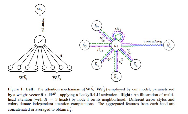
    • (this paper) use \(a\) as FFNN, parameterized by \(\overrightarrow{\mathbf{a}} \in \mathbb{R}^{2 F^{\prime}}\)+ LeakyReLU
  • \(\alpha_{i j}=\operatorname{softmax}_{j}\left(e_{i j}\right)=\frac{\exp \left(e_{i j}\right)}{\sum_{k \in \mathcal{N}_{i}} \exp \left(e_{i k}\right)}\).
  • \(\alpha_{i j}=\frac{\exp \left(\operatorname{LeakyReLU}\left(\overrightarrow{\mathbf{a}}^{T}\left[\mathbf{W} \vec{h}_{i} \mid \mid \mathbf{W} \vec{h}_{j}\right]\right)\right)}{\sum_{k \in \mathcal{N}_{i}} \exp \left(\text { LeakyReLU }\left(\overrightarrow{\mathbf{a}}^{T}\left[\mathbf{W} \vec{h}_{i} \mid \mid \mathbf{W} \vec{h}_{k}\right]\right)\right)}\).
• Result (final output features) for every node
  • (1-head) \(\vec{h}_{i}^{\prime}=\sigma\left(\sum_{j \in \mathcal{N}_{i}} \alpha_{i j} \mathbf{W} \vec{h}_{j}\right)\).
    • \(\mathbf{h}^{\prime}\) consists of \(F^{\prime}\) features
  • (multi(K)-head + concatenate) \(\vec{h}_{i}^{\prime}= \mid \mid _{k=1}^{K} \sigma\left(\sum_{j \in \mathcal{N}_{i}} \alpha_{i j}^{k} \mathbf{W}^{k} \vec{h}_{j}\right)\)
    • \(\mathbf{h}^{\prime}\) consists of \(K F^{\prime}\) features
  • (multi(K)-head + average) \(\vec{h}_{i}^{\prime}=\sigma\left(\frac{1}{K} \sum_{k=1}^{K} \sum_{j \in \mathcal{N}_{i}} \alpha_{i j}^{k} \mathbf{W}^{k} \vec{h}_{j}\right)\)
    • in the final layer
    • \(\mathbf{h}^{\prime}\) consists of \(F^{\prime}\) features