
Interpretability Beyond Feature Atribution : Quantitative Testing with Concept Activation Vectors (TCAV) (2017)
Contents
- Abstract
- Introduction
- Related Work
- Interpretability methods
- Interpretability methods in NN
- Linearity in NN and latent dimensions
- Methods
- User-defined Concepts as Sets of Examples
- CAVs ( Concept Activation Vectors )
- Directional Derivatives and Conceptual Sensitivity
- TCAV ( Testing with CAVs )
0. Abstract
Interpretation of DL = challenging! WHY?
\(\rightarrow\) OPERATE on low-level feature ( not on high-level concept )
Introduce CAVs (Concept Activation Vectors)
-
provide an interpretation of NN’s internal state in terms of human-friendly concepts
-
key idea : view high-dim internal state of NN as an aid
1. Introduction
Interpretability를 바라보는 대표적인 관점
- describe prediction “in terms of INPUT FEATURES”
이의 문제점?
-
1) 대부분의 ML모델은 주로 feature ( ex. pixel value ) 상에서 operate
( \(\neq\) 인간이 이해 가능한 high level concept )
-
2) model’s internal values ( ex. neural activations ) : 너무 incomprehensible
Notation
-
state of ML model : \(E_m\) ( spanned by basis vectors \(e_m\) )
-
vector space of human : \(E_h\)
( 여기서 \(E_h\)는 input feature /training data로 국한되지 않고, user-provided data도 OK )
결국, 우리가 “interpretation”을 한다는 것은, \(g : E_m \rightarrow E_h\)를 찾는 것!
( 여기서 \(g=\) linear일 경우, linear interpretability )
Concept Activation Vector (CAV)
- \(E_m\)과 \(E_h\)를 translate하는 방법
- derive CAVs by training a linear classifier between concept’s examples & random counter examples
quantitative Testing with CAV (TCAV)
-
이 논문의 최종 결과! new linear interpretability method
-
use directional derivatives
to quantify the model prediction’s sensitivity to an underlying HIGH-level concept
-
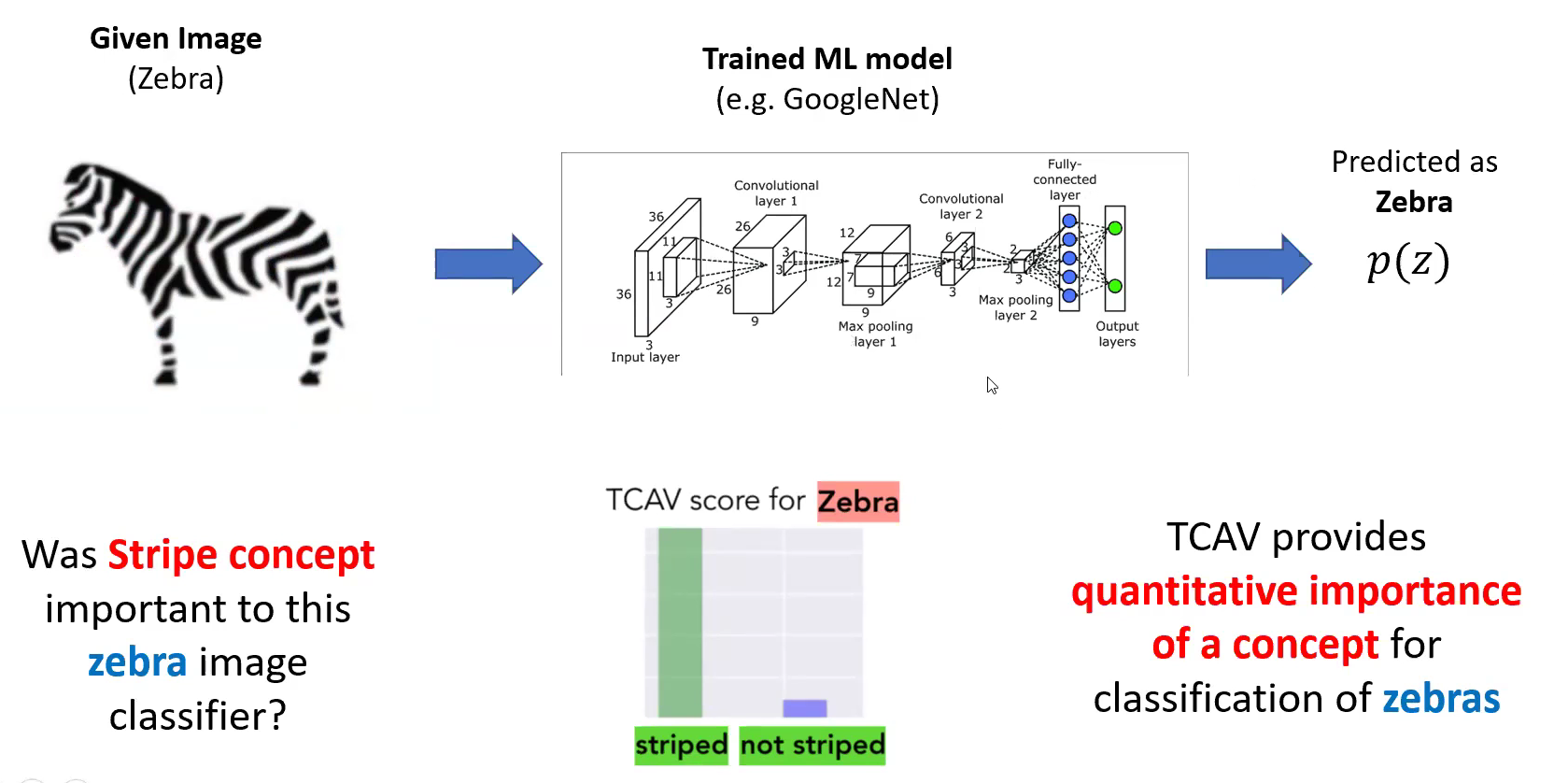
ex) “얼룩말” 사진
- user-defined set of examples : “striped” (줄무늬가 있는)
- TCAV는 “striped”라는 concept이 “얼룩말”이라는 prediction을 낸 영향을 quantify할 수 있다.
TCAV의 goals
- 1) Accessibility : ML 전문가가 아니더라도 OK
- 2) Customization : adapts to ANY concept
- 3) Plug-in readiness : retraining (X)
- 4) Global quantification : interpret ENTIRE CLASSES (O), individual datapoints (X)
2. Related Work
-
2-1) overview of interpretability methods
- 2-2) methods specific to NN
- 2-3) methods that leverage the local linearity of NNs
2-1) Interpretability methods
interpretability를 얻기 위한 2가지 옵션
- [옵션 1] interpretable model로 모델을 국한시키기
- 어려운 점 ) high performance 어려워
- [옵션 2] 모델을 post-process하여 insight를 얻기
- 어려운 점 ) ensure the explanation correctly reflects model’s complex internals
interpretability를 얻기 위한 method의 트렌드
-
method that can be applied without retraining or without modifying the network
-
use generated explanation as input & check network’s output for validation
( 주로 perturbation-based / sensitivity analysis-based interpretability methods 에서 사용 )
Perturbation-based
-
use data/features as a form of perturbation
& check response changes
-
maintain consistency..
-
1) locally ( data point & neighbors에서 explanation이 true )
-
2) globally ( 거의 모은 data point ~ )
\(\rightarrow\) TCAV는 global perturbation method
-
2-2) Interpretability methods in NN
TCAV의 목표 : interpret high-dim \(E_m\)
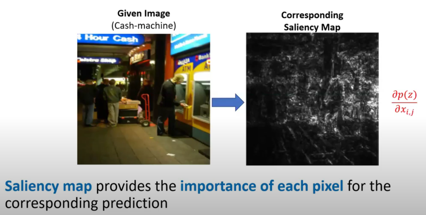
Saliency methods :
-
popular local explanation methods for image classification
-
produce a map showing how important each pixel is!
Saliency Map :
( 출처 : https://www.youtube.com/watch?v=-y0oghbEHMM&t=1127s )
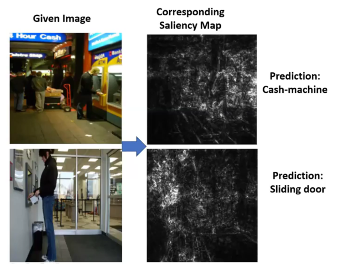
limitations of Saliency Map
- 1) conditioned on only ONE picture
- 2) users have NO CONTROL over what concepts of interest these maps pick up on
- 3) vulnerable to adversarial attacks
2-3) Linearity in NN and latent dimensions
1) Linear combination of neurons encode meaningful information!
- meaningful directions can be efficiently learned by simple linear classifiers
2) Mapping latent dimensions to human concepts
이 논문의 아이디어
-
compute directional derivatives along these learned directions
( 각 direction의 importance 확인 위해! )
4. Methods
ideas & methods
-
(a) how to use directional derivatives to quantify sensitivity of predictions for different conepts
-
(b) how to compute the final quantitative explanation ( without retraining )
quantitative explanation : 해당 concept이 해당 예측결과를 내는데에 있어서 얼마나 중요한 역할을 했는지 정량화!
( 주의 : 여기서 concept은 training 과정이나, label과는 전혀 무관! 아예 모델 train 완료된 이후, 사용하는 개념! )
Notation
- input : \(x \in \mathbb{R}^{n}\)
- feedforward layer \(l\) with \(m\) neurons
- \(f_{l}: \mathbb{R}^{n} \rightarrow \mathbb{R}^{m}\).
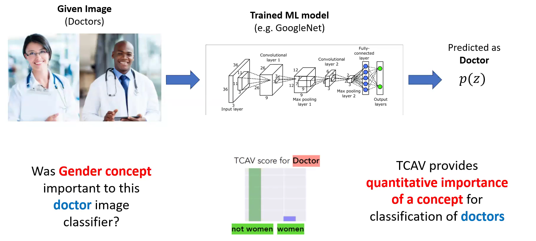
Goal of TCAV
( 출처 : https://www.youtube.com/watch?v=-y0oghbEHMM&t=1127s )
3-1) User-defined Concepts as Sets of Examples
[1단계] concept 정의하기!
- find an independent dataset with concept labeled
- 두 종류의 dataset을 구한다
- 1) concept set과 관련된 dataset ( ex. “줄무늬” 관련 사진 )
- 2) random dataset ( ex. 아무 사진 )
3-2) CAVs ( Concept Activation Vectors )
[2단계] 위에서 구한 set of examples에서, 해당 concept을 나타내는 vector 찾기
-
HOW? consider the activations in layer \(l\), produced by input examples that
in the concept set vs random examples
[3단계] CAV (concept activation vector) 정의하기
- 정의) normal to a hyperplane, separating WITH/WITHOUT CONCEPT
- concept : \(C\)
- positive set of example inputs : \(P_C\)
- negative set : \(N\)
- binary linear classifier 학습 ( distinguish between the layer activations of two sets )
- \(\left\{f_{l}(\boldsymbol{x}): \boldsymbol{x} \in P_{C}\right\}\).
- \(\left\{f_{l}(\boldsymbol{x}): \boldsymbol{x} \in N\right\}\).
3-3) Directional Derivatives and Conceptual Sensitivity
Saliency map 복습 ( 위의 2-2) 참조하기 )
- use gradients of logit values w.r.t individual input features ( ex. pixel )
- 즉, 다음을 계산 : \(\frac{\partial h_{k}(\boldsymbol{x})}{\partial \boldsymbol{x}_{a, b}}\)
- \(h_{k}(\boldsymbol{x})\) : logit for a data point \(\boldsymbol{x}\) for class \(k\)
- \(\boldsymbol{x}_{a, b}\) : pixel at position \((a, b)\) in \(\boldsymbol{x}\).
CAV와 directional derivatives를 이용함으로써…
-
sensitivity of predictions to changes in inputs towards the direction of a concept를 파악 가능!
-
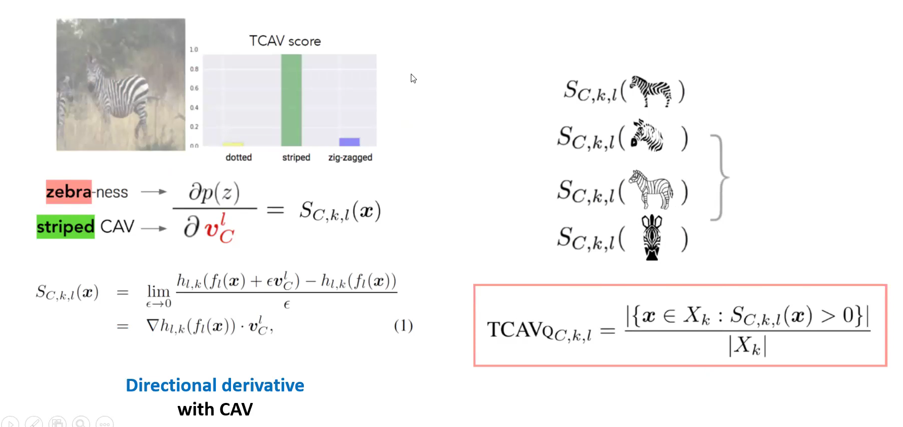
“Conceptual Sensitivity” :
\(\begin{aligned} S_{C, k, l}(\boldsymbol{x}) &=\lim _{\epsilon \rightarrow 0} \frac{h_{l, k}\left(f_{l}(\boldsymbol{x})+\epsilon \boldsymbol{v}_{C}^{l}\right)-h_{l, k}\left(f_{l}(\boldsymbol{x})\right)}{\epsilon} \\ &=\nabla h_{l, k}\left(f_{l}(\boldsymbol{x})\right) \cdot \boldsymbol{v}_{C}^{l}, \end{aligned}\).
where \(h_{l, k}: \mathbb{R}^{m} \rightarrow \mathbb{R}\).
3-4) TCAV ( Testing with CAVs )
-
위에서 CAV & directional derivatives를 통해 구한 “Conceptual Sensitivity”( = \(S_{C, k, l}(\boldsymbol{x})\) ) 사용
-
notation
- \(k\) : class label
- \(X_k\) : class label \(k\)를 가진 모든 inputs
-
TCAV score : \(\operatorname{TCAV}_{\mathrm{Q} C, k, l}=\frac{ \mid \left\{\boldsymbol{x} \in X_{k}: S_{C, k, l}(\boldsymbol{x})>0\right\} \mid }{ \mid X_{k} \mid }\).
-
the fraction of \(k\) -class inputs whose \(l\) -layer activation vector was POSITIVELY influenced by concept \(C\)
- only depends on “sign of \(\operatorname{TCAV}_{Q, k, l}\)”
- easily interpreted & globally
-
( 출처 : https://www.youtube.com/watch?v=-y0oghbEHMM&t=1127s )
3-5) Sensitivity of TCAV scores
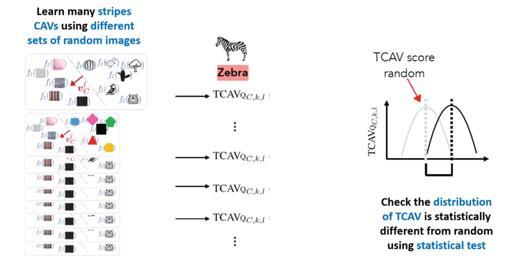
( 출처 : https://www.youtube.com/watch?v=-y0oghbEHMM&t=1127s )
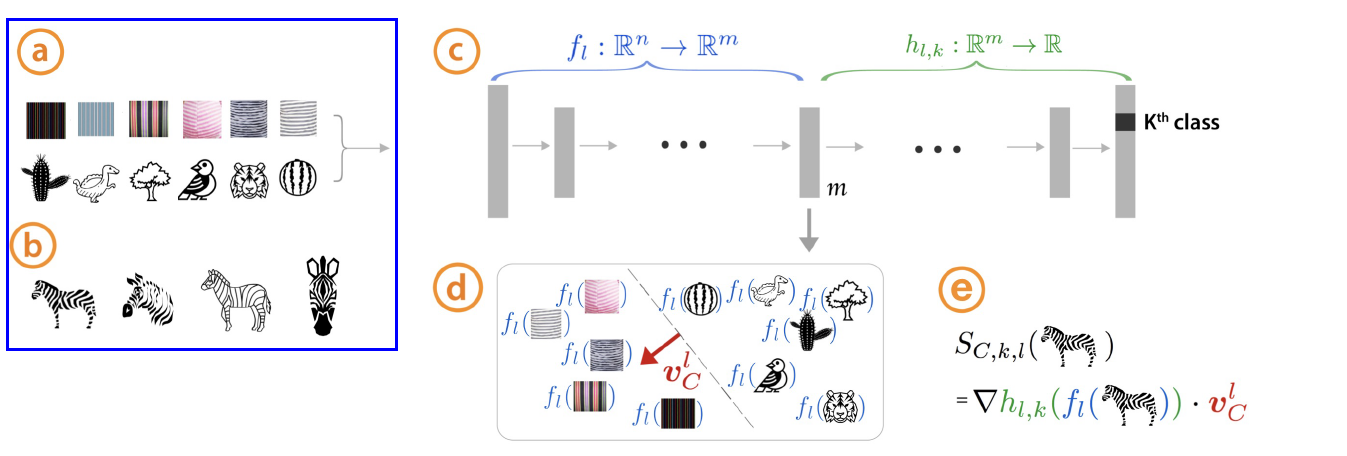
알고리즘 요약
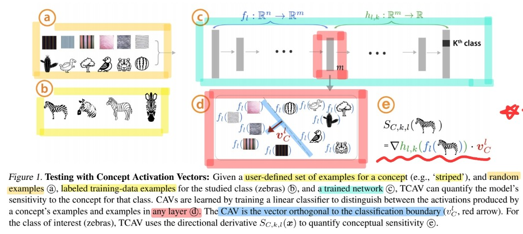
-
정의한 concept : striped (줄무늬 있는)
-
(a) random examples
-
(b) labeled training-data exxamples ( 줄무늬 있는 얼룩말 )
-
(c) trained network
-
(d) 위의 (c)에서, \(l\) 번쨰째 layer를 뽑아냄 ( 차원 : \(m\) 차원 )
- 이를 통해 (a) & (b)를 구분하는 linear classifier
- 여기서 hyperplane에 직교하는 선이 CAV
-
(e) TCAV