
Matching Networks for One Shot Learning
Contents
- Abstract
- Introduction
- Model
- Model Architecture
- Training Strategy
- Related Work
- MANN
- Metric Learning
0. Abstract
적은 수의 데이터로부터 배우는 것 : challenging!
standard DL 방법론으로 풀기 쉽지 않다!
이 논문에서 제안한 Matching Network는 아래의 1) + 2)
- 1) “METRIC learning” based on deep neural features
- 2) augment NN with “EXTERNAL” memories
small “labeled” SUPPORT set을 통해 network를 학습
그런 뒤, unlabelled example를 위의 SUPPORT set의 label 중 하나로 할당
1. Introduction
( NN과 같이 ) 우리가 주로 사용하는 모델은 parametric model
이러한 모델의 문제점들 : (meta learning 관점에서)
- 1) slow in learning
- 2) large dataset \(\rightarrow\) require many weight updates
이에 반해, non-parametric model들은..
- 1) rapid
- 2) not suffer from catastrophic forgetting
- example : kNN
Matching Nets (MN)의 novelty :
-
측면 1) modeling
- attention & memory 사용
-
측면 2) training procedure
-
test & train condition이 서로 match
( 즉, test 단계에 실제로 class 별 few example 밖에 없으니까, train 단계 때도 few example로 학습 )
-
2. Model
- NON-parametric한 모델
- 2가지 핵심 특징
- 1) NN augmented with memory
- 2) training strategy, tailored for one-shot learning from support set \(S\)
2-1. Model Architecture
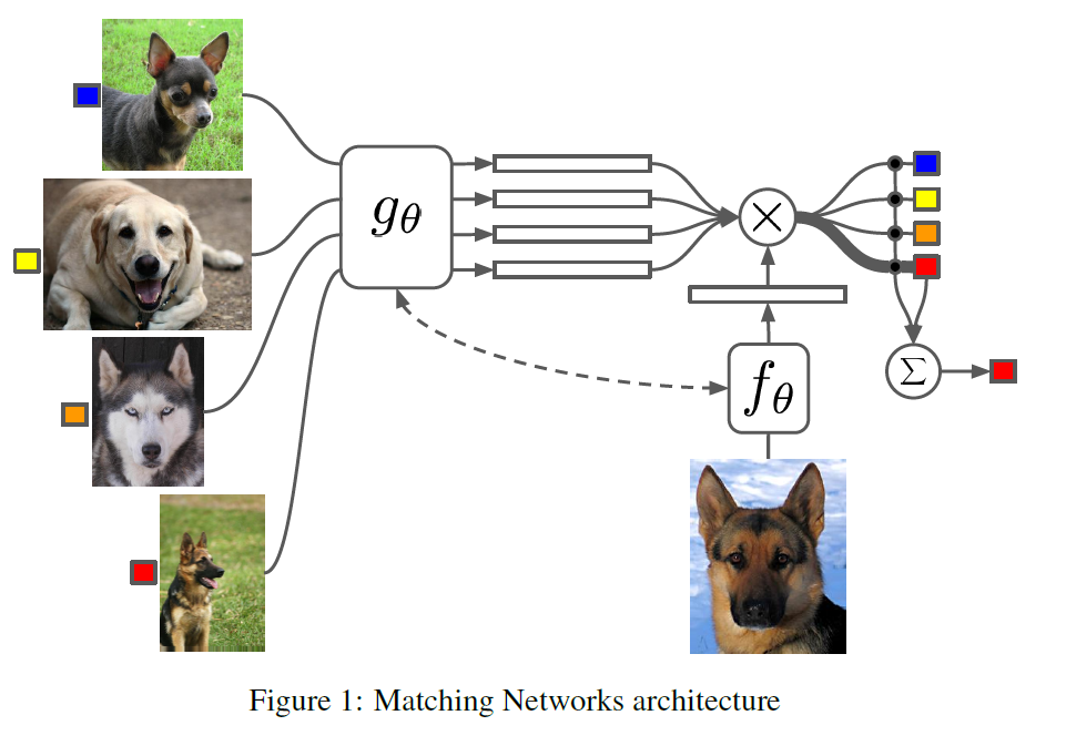
-
Neural Attention mechanism : memory matrix 사용
- 처음 보는 class가 등장해도, “기존의 network의 변화 없이도” 예측 가능!
- \(\mathcal{S}=\left\{\left(x_{i}, y_{i}\right)\right\}_{i=1}^{k}\) 를 사용하여 \(P(\hat{y} \mid \hat{x}, \mathcal{S})\)를 예측
- 여기서 사용하는 모델 : NN
- 최종 예측 class : \(\text{argmax}_y P(y \mid \hat{x}, \mathcal{S})\)
- \(\hat{y}=\sum_{i=1}^{k} a\left(\hat{x}, x_{i}\right) y_{i}\).
- attention을 통해 유사도 만큼을 weight로써 사용
Attention
\(a\left(\hat{x}, x_{i}\right)=\frac{e^{c\left(f(\hat{x}), g\left(x_{i}\right)\right)}}{\sum_{j=1}^{k} e^{c\left(f(\hat{x}), g\left(x_{i}\right)\right)}}\).
- \(c\) : 코사인 유사도
- \(f\) & \(g\) : embedding function ( deep convolutional network )
Full Context Embeddings
-
Matching Net의 핵심은 “one-shot learning”에 특화되어 있다는 것!
-
\(f\)와 \(g\)는 classification에서 높은 accuracy를 얻도록 데이터를 feature space \(X\)로 embedding 해줌
-
새로운 embedding 구조도 가능!
( Support set 내에서의 연관성도 반영하고자 )
-
기존 ) \(g\left(x_{i}\right), f(\hat{x})\)
\(\rightarrow\) \(f, g\) 을 사용해 임베딩을 생성하는 당시에는 \(\mathcal{S}\) 가 고려되지 않음
-
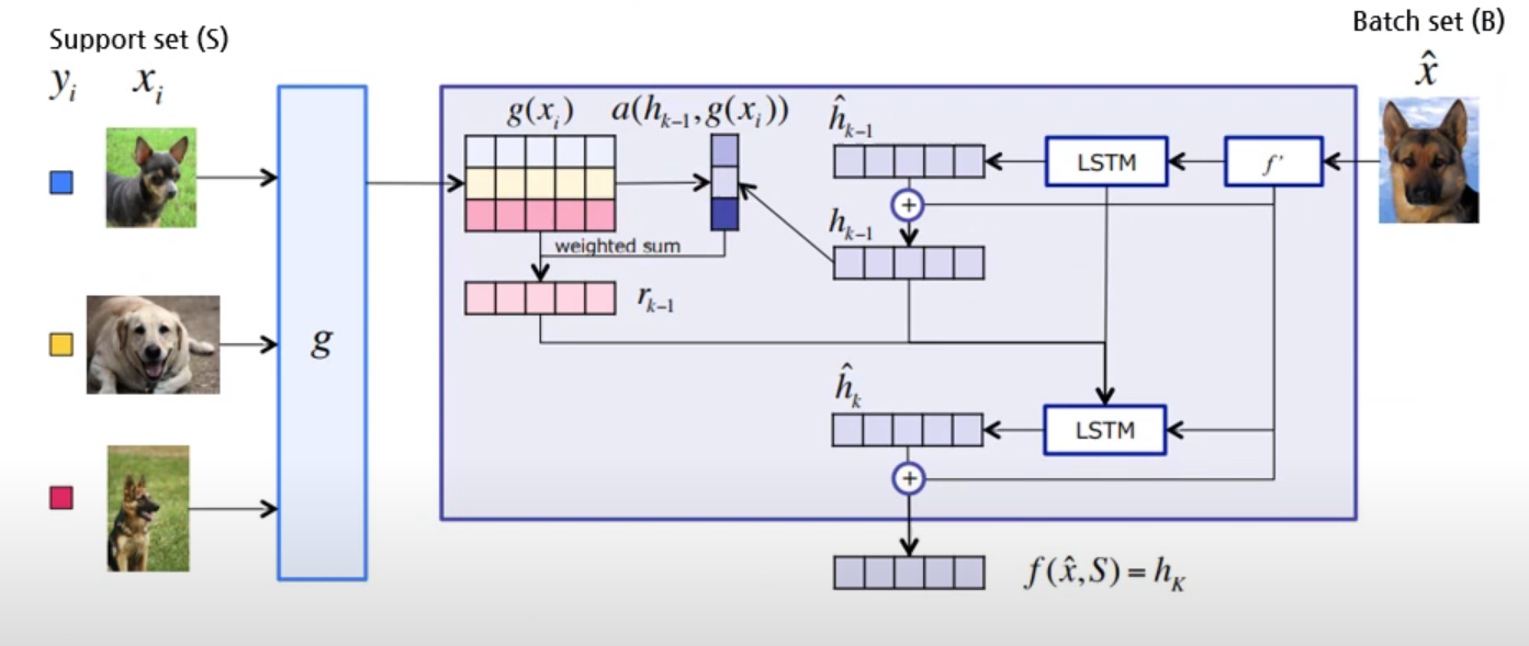
제안 ) \(g\left(x_{i}, \mathcal{S}\right), f(\hat{x}, \mathcal{S})\)
\(\rightarrow\) \(\mathcal{S}\)의 맥락 속에서 \(x\)들을 embedding한다고 생각하면 됨
-
\(g\) : biLSTM
-
\(f\) : attention ( \(\left.f(\hat{x}, \mathcal{S})=\operatorname{attLSTM}\left(f^{\prime}(\hat{x}), g(\mathcal{S}), K\right)\right)\) )
( \(f'(\hat{x})\) : features which are input to LSTM )
-
-
g function ( biLSTM )
- support set 임베딩
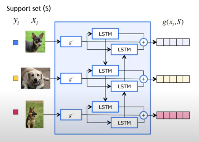
\(\begin{aligned} &\vec{h}_{i}, \vec{c}_{i}=\operatorname{LSTM}\left(g^{\prime}\left(x_{i}\right), \vec{h}_{i-1}, \vec{c}_{i-1}\right) \\ &\stackrel{r}{h}_{i}, \bar{c}_{i}=\operatorname{LSTM}\left(g^{\prime}\left(x_{i}\right), \stackrel{h}{h}_{i+1}, \bar{c}_{i+1}\right) \\ &g\left(x_{i}, S\right)=\vec{h}_{i}+\stackrel{\leftarrow}{h}_{i}+g^{\prime}\left(x_{i}\right) \end{aligned}\).
f function ( Attention)
- batch set 임베딩
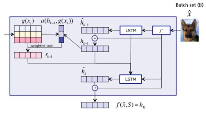
\(\begin{aligned} \hat{h}_{k}, c_{k} &=\operatorname{LSTM}\left(f^{\prime}(\hat{x}),\left[h_{k-1}, r_{k-1}\right], c_{k-1}\right) \\ h_{k} &=\hat{h}_{k}+f^{\prime}(\hat{x}) \\ r_{k-1} &=\sum_{i=1}^{|S|} a\left(h_{k-1}, g\left(x_{i}\right)\right) g\left(x_{i}\right) \end{aligned}\).
\(a\left(h_{k-1}, g\left(x_{i}\right)\right)=\operatorname{softmax}\left(h_{k-1}^{T} g\left(x_{i}\right)\right)\).
\(\begin{aligned} f(\hat{x}, S) &=\operatorname{attLSTM}\left(f^{\prime}(\hat{x}), g(S), K\right) =h_{K} \end{aligned}\).
Full Context Embedding 최종
-
\(P\left(\hat{y}_{k}=1 \mid \hat{x}, \delta\right)=\sum_{i=1}^{k} a\left(\hat{x}, x_{i}\right) y_{i}\).
-
\(a(\hat{x}, x)=\frac{\exp (c(f(\hat{x}), g(x)))}{\sum_{i=1}^{K} \exp \left(c\left(f(\hat{x}), g\left(x_{i}\right)\right)\right)}\).
2-2. Training Strategy
“set-to-set 패러다임 augmented with attention”
Notation
-
\(\mathcal{T}\) : task 모음
-
\(\mathcal{L}\) : label 모음 ( \(L \sim T\) )
Episode ( training 알고리즘 )
-
1) \(T\) 에서 \(L\)을 샘플한다 ( \(L \sim T\) ) … ex) \(L=\)(cat, dog)
-
2) \(L\)을 사용하여,
- support set \(S\)와 (=학습용)
- batch \(B\)를 샘플 (=테스트용)
-
3) \(B\)에 대한 error를 최소화하도록 하는 모델을 \(S\)를 통해 학습
objective function : \(\theta=\arg \max _{\theta} \mathbb{E}_{\mathcal{L} \sim T}\left[\mathbb{E}_{S \sim \mathcal{L}, B \sim \mathcal{L}}\left[\sum_{(x, y) \in B} \log P_{\theta}(y \mid x, S)\right]\right]\).
3. Related Work
3-1. MANN
( 논문 리뷰 : https://seunghan96.github.io/meta/study/study-(meta)(paper-1)-Meta-learning-with-Memory-Augmented-Neural-Networks/ 참고하기 )
-
Memory Augmented Neural Network (MANN)의 패러다임을 차용
( LSTM learnt to learn quickly from data presented sequentially )
-
차이점은, data를 하나의 “set”으로 바라봤다는 점
3-2. Metric Learning
- NCA (Neighborhood Component Analysis)의 패러다임을 차용 + non-linear version
- 핵심 ) 주변 구성 요소 분석을 통한 차원 축소 ( embedding )
Reference
-
https://www.youtube.com/watch?v=SW0cgNZ9eZ4