
Prototypical Networks for Few-shot Learning
Contents
- Abstract
- Introduction
- Prototypical Networks
- Notation
- Model
- Prototypical Networks as Mixture Density Estimation
- Reinterpretation as Linear Model
- Comparison to Matching Networks
- Design Choices
0. Abstract
Classifier must GENERALIZE to new classes, NOT SEEN in training set, given only SMALL NUMBER of examples of each new class
-
train ) 강아지 5만장, 고양이 5만장, 토끼 5만장
-
test ) 거북이 10장…??
( 이걸로만 train하기엔 overfitting 문제 )
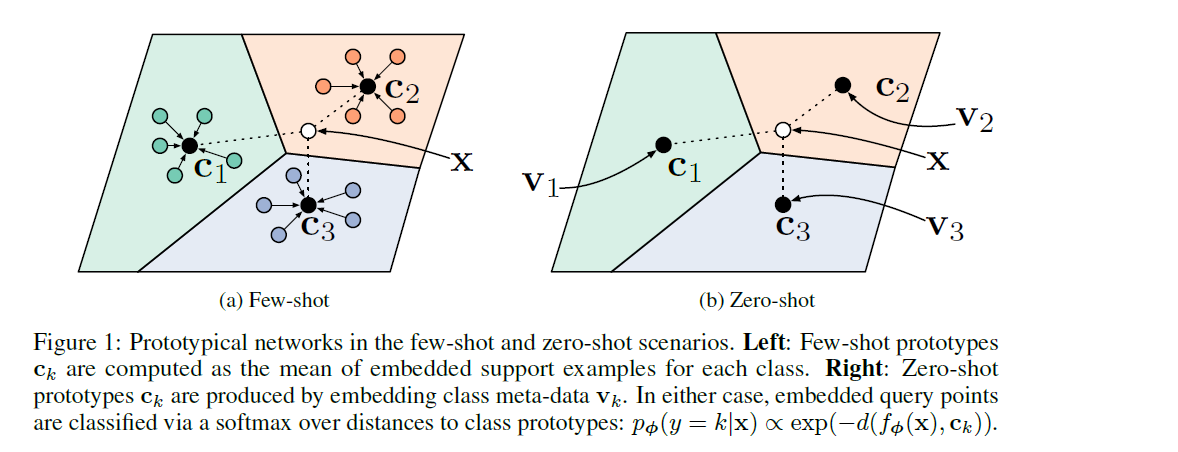
Prototypical Network 핵심 :
- compute distances to prototype representations of each class
1. Introduction
Few shot Learning의 2가지 recent approaches
- 1) Matching Networks
- 2) meta-LSTM
\(\rightarrow\) 둘 다 여전히 overfitting issue 남아있어
Prototypical Networks
-
idea ) 모든 class 별로, 각각을 대표하는 single prototype representation이 있다!
- NN을 사용한 non-linear mapping
- class’s prototype = mean of Support set in the embedding space
2. Prototypical Networks
2-1. Notation
[Support set] \(S=\left\{\left(\mathbf{x}_{1}, y_{1}\right), \ldots,\left(\mathbf{x}_{N}, y_{N}\right)\right\}\)
- \(N\) labeled samples
- \[\mathbf{x}_{i} \in \mathbb{R}^{D}\]
- \[y_{i} \in\{1, \ldots, K\}\]
- \(S_{k}\) : examples labeled with class \(k\).
2-2. Model
prototype : \(M\)-dimension의 representation \(\mathbf{c}_{k} \in \mathbb{R}^{M}\)
-
embedding function \(f_{\phi}: \mathbb{R}^{D} \rightarrow \mathbb{R}^{M}\) 통해 학습한다
-
각 prototype은, 각 class 별 mean vector of the embedded support points
- \(\mathbf{c}_{k}=\frac{1}{ \mid S_{k} \mid } \sum_{\left(\mathbf{x}_{i}, y_{i}\right) \in S_{k}} f_{\phi}\left(\mathbf{x}_{i}\right)\).
Model : \(p_{\boldsymbol{\phi}}(y=k \mid \mathbf{x})=\frac{\exp \left(-d\left(f_{\boldsymbol{\phi}}(\mathbf{x}), \mathbf{c}_{k}\right)\right)}{\sum_{k^{\prime}} \exp \left(-d\left(f_{\boldsymbol{\phi}}(\mathbf{x}), \mathbf{c}_{k^{\prime}}\right)\right)}\)
- \(d\) : distance function
- 가장 가까운 prototype의 class에 귀속시키기
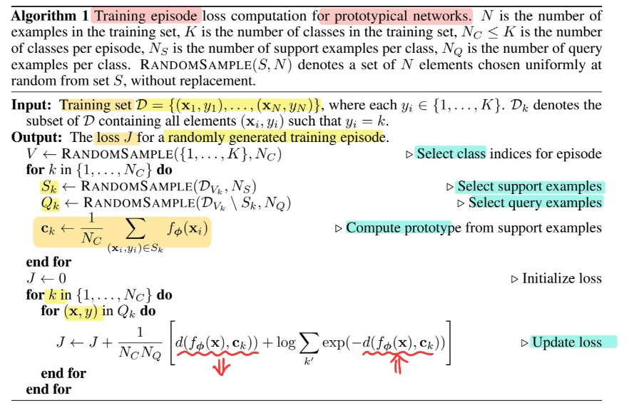
[ Training Procedure ]
- loss function : NLL
- \(J(\phi)=-\log p_{\phi}(y=k \mid \mathbf{x})\).
- training episode :
- step 1) randomly select subset of classes from training set
- step 2) choosing a subset of examples within each class
- Support set & Query set으로 나눠
2-3. Prototypical Networks as Mixture Density Estimation
distance function의 종류 : regular Bregman divergences
-
이를 사용할 경우, Prototypical Networks = support set에 Mixture Density Estimation하는 것
( with exponential family density )
-
regular Bregman divergences :
- \(d_{\varphi}\left(\mathbf{z}, \mathbf{z}^{\prime}\right)=\varphi(\mathbf{z})-\varphi\left(\mathbf{z}^{\prime}\right)-\left(\mathbf{z}-\mathbf{z}^{\prime}\right)^{T} \nabla \varphi\left(\mathbf{z}^{\prime}\right)\).
-
대표적인 ex) Euclidean distance & Mahalanobis distance
Prototype computation as MDE
-
Prototype computation = hard clustering on support set ( one cluster per one class )
-
\(p_{\psi}(\mathbf{z} \mid \boldsymbol{\theta})\) 를 exponential family로 잡을 경우
-
\(p_{\psi}(\mathbf{z} \mid \boldsymbol{\theta})=\exp \left\{\mathbf{z}^{T} \boldsymbol{\theta}-\psi(\boldsymbol{\theta})-g_{\psi}(\mathbf{z})\right\}=\exp \left\{-d_{\varphi}(\mathbf{z}, \boldsymbol{\mu}(\boldsymbol{\theta}))-g_{\varphi}(\mathbf{z})\right\}\).
\(p(\mathbf{z} \mid \mathbf{\Gamma})=\sum_{k=1}^{K} \pi_{k} p_{\psi}\left(\mathbf{z} \mid \boldsymbol{\theta}_{k}\right)=\sum_{k=1}^{K} \pi_{k} \exp \left(-d_{\varphi}\left(\mathbf{z}, \boldsymbol{\mu}\left(\boldsymbol{\theta}_{k}\right)\right)-g_{\varphi}(\mathbf{z})\right)\).
-
inference 단계 :
\[p(y=k \mid \mathbf{z})=\frac{\pi_{k} \exp \left(-d_{\varphi}\left(\mathbf{z}, \boldsymbol{\mu}\left(\boldsymbol{\theta}_{k}\right)\right)\right)}{\sum_{k^{\prime}} \pi_{k^{\prime}} \exp \left(-d_{\varphi}\left(\mathbf{z}, \boldsymbol{\mu}\left(\boldsymbol{\theta}_{k}\right)\right)\right)}\] -
위 식에서 \(f_{\phi}(\mathrm{x})=\mathrm{z}\) and \(\mathbf{c}_{k}=\boldsymbol{\mu}\left(\boldsymbol{\theta}_{k}\right)\)로 놓으면, 기존 알고리즘과 동일
-
2-4. Reinterpretation as a Linear Model
Euclidean distance ( \(d\left(\mathbf{z}, \mathbf{z}^{\prime}\right)= \mid \mid \mathbf{z}-\mathbf{z}^{\prime} \mid \mid ^{2}\) ) 를 사용할 경우,
-
\(p_{\boldsymbol{\phi}}(y=k \mid \mathbf{x})=\frac{\exp \left(-d\left(f_{\boldsymbol{\phi}}(\mathbf{x}), \mathbf{c}_{k}\right)\right)}{\sum_{k^{\prime}} \exp \left(-d\left(f_{\boldsymbol{\phi}}(\mathbf{x}), \mathbf{c}_{k^{\prime}}\right)\right)}\) 는 linear model로 볼 수 있음
-
\(- \mid \mid f_{\phi}(\mathrm{x})-\mathrm{c}_{k} \mid \mid ^{2}=-f_{\phi}(\mathrm{x})^{\top} f_{\phi}(\mathrm{x})+2 \mathrm{c}_{k}^{\top} f_{\phi}(\mathrm{x})-\mathrm{c}_{k}^{\top} \mathrm{c}_{k}\).
-
여기서, \(k\)와 무관한 term 빼고 보면…
\(2 \mathbf{c}_{k}^{\top} f_{\phi}(\mathbf{x})-\mathbf{c}_{k}^{\top} \mathbf{c}_{k}=\mathbf{w}_{k}^{\top} f_{\phi}(\mathbf{x})+b_{k}\).
- \[\text { where } \mathbf{w}_{k}=2 \mathbf{c}_{k} \text { and } b_{k}=-\mathbf{c}_{k}^{\top} \mathbf{c}_{k}\]
-
-
Euclidean distnace는 effective choice다!
( linear model이지만, embedding function에서 non-linearity 캐치하므로! )
2-5. Comparison to Matching Networks
- [MN] weighted nearest neighbor classifier
- [PN] linear classifier when squared Euclidean distance is used
One-shot learning의 경우, \(\mathbf{c}_k=\mathbf{x}_k\) \(\rightarrow\) MN=PN
2-6. Design Choices
(a) Distance Metric
-
MN과 PN 모두 어떠한 distance function OK
-
하지만, 일반적으로 cosine distance보다 Euclidean distance가 더 좋은 성능
( cosine distance는 Bregman divergence에 안속해서, MDE 불가 )
(b) Episdoe Composition
-
\(N_c\) class & \(N_s\) support points per class 설정
ex) 5-way 1-shot learning : \(N_c = 5, N_s = 1\)
-
Train 시, 더 높은 \(N_c\) 사용하면 더 beneficial한 것을 확인함
-
Test시, train과 동일한 “shot”을 사용하는것이 best