(PRML) Ch10.Approximate Inference

( Skip the basic parts + not important contents )

10. Approximate Inference

Important task in probabilistic models = “evaluation of the posterior” (\(P(\mathbf{Z}\mid\mathbf{X})\) )

EM algorithm

• evaluate the expectation of complete-data log likelihood, w.r.t posterior of latent variable

But in practice….

• problem 1) dimension of latent space : TOO HIGH
• problem 2) not analytically tractable
  • continuous ) may not have closed-form
  • discrete ) always possible in principle, but exponentially many hidden states \(\rightarrow\)expensive

Thus, we need “APPROXIMATION”….fall into 2 classes

• 1) stochastic approx

  • MCMC ( Ch.11 )
  • given infinite computational resource, generate exact result!
  • but computationally demanding \(\rightarrow\) limited to small-scale problems

• 2) deterministic approx

  • scale well to large applications

  • based on “analytical approximations” to posterior

    ( ex. factorizes with Gaussian )

  • Laplace approximation

    ( based on local Gaussian approximation to a mode of distn )

  • Variational Inference, Expectation Propagation

10-1. Variational Inference

“approximate \(p\) with simple distribution \(q\) “

10-1-1. Factorized distribution

assume that \(q\) factorizes as…

• \(q(\mathrm{Z})=\prod_{i=1}^{M} q_{i}\left(\mathrm{Z}_{i}\right)\).

Make Lower bound \(L(q)\) largest

\(\begin{aligned} \mathcal{L}(q) &=\int \prod_{i} q_{i}\left\{\ln p(\mathbf{X}, \mathbf{Z})-\sum_{i} \ln q_{i}\right\} \mathrm{d} \mathbf{Z} \\ &=\int q_{j}\left\{\int \ln p(\mathbf{X}, \mathbf{Z}) \prod_{i \neq j} q_{i} \mathrm{~d} \mathbf{Z}_{i}\right\} \mathrm{d} \mathbf{Z}_{j}-\int q_{j} \ln q_{j} \mathrm{~d} \mathbf{Z}_{j}+\text { const } \\ &=\int q_{j} \ln \tilde{p}\left(\mathbf{X}, \mathbf{Z}_{j}\right) \mathrm{d} \mathbf{Z}_{j}-\int q_{j} \ln q_{j} \mathrm{~d} \mathbf{Z}_{j}+\text { const } \end{aligned}\).

• define new distribution \(\tilde{p}\left(\mathbf{X}, \mathbf{Z}_{j}\right)\)
  • \(\ln \tilde{p}\left(\mathbf{X}, \mathbf{Z}_{j}\right)=\mathbb{E}_{i \neq j}[\ln p(\mathbf{X}, \mathbf{Z})]+\operatorname{const.}\).
  • where \(\mathbb{E}_{i \neq j}[\ln p(\mathbf{X}, \mathbf{Z})]=\int \ln p(\mathbf{X}, \mathbf{Z}) \prod_{i \neq j} q_{i} \mathrm{~d} \mathbf{Z}_{i}\)

Maximizing lower bound (\(L(q)\) ) = minimizing KL-divergence

\(\rightarrow\) occurs when \(q_{j}\left(\mathbf{Z}_{j}\right)=\tilde{p}\left(\mathbf{X}, \mathbf{Z}_{j}\right) .\)

Thus, optimal solution

• \[\ln q_{j}^{\star}\left(\mathbf{Z}_{j}\right)=\mathbb{E}_{i \neq j}[\ln p(\mathbf{X}, \mathbf{Z})]+\text { const. }\]
  • constant : set by normalizing the distribution
• \(q_{j}^{\star}\left(\mathbf{Z}_{j}\right)=\frac{\exp \left(\mathbb{E}_{i \neq j}[\ln p(\mathbf{X}, \mathbf{Z})]\right)}{\int \exp \left(\mathbb{E}_{i \neq j}[\ln p(\mathbf{X}, \mathbf{Z})]\right) \mathrm{d} \mathbf{Z}_{j}}\).

10-1-2. Properties of factorized approximations

one approach of VI = based on “factorized approximation”

• ex) using a factorized Gaussian

Example

• \(p(\mathbf{z})=\mathcal{N}\left(\mathbf{z} \mid \boldsymbol{\mu}, \boldsymbol{\Lambda}^{-1}\right)\)., where \(\mathrm{z}=\left(z_{1}, z_{2}\right)\)
  • mean and variance : \(\boldsymbol{\mu}=\left(\begin{array}{c} \mu_{1} \\ \mu_{2} \end{array}\right), \quad \boldsymbol{\Lambda}=\left(\begin{array}{ll} \Lambda_{11} & \Lambda_{12} \\ \Lambda_{21} & \Lambda_{22} \end{array}\right)\).
• \(q(\mathrm{z})=\) \(q_{1}\left(z_{1}\right) q_{2}\left(z_{2}\right)\)

Only retain those terms that depend on \(z_1\)

( all other terms are absorbed to normalizing constant )

\(\begin{aligned} \ln q_{1}^{\star}\left(z_{1}\right) &=\mathbb{E}_{z_{2}}[\ln p(\mathbf{z})]+\text { const } \\ &=\mathbb{E}_{z_{2}}\left[-\frac{1}{2}\left(z_{1}-\mu_{1}\right)^{2} \Lambda_{11}-\left(z_{1}-\mu_{1}\right) \Lambda_{12}\left(z_{2}-\mu_{2}\right)\right]+\mathrm{const} \\ &=-\frac{1}{2} z_{1}^{2} \Lambda_{11}+z_{1} \mu_{1} \Lambda_{11}-z_{1} \Lambda_{12}\left(\mathbb{E}\left[z_{2}\right]-\mu_{2}\right)+\mathrm{const.} \end{aligned}\).

Therefore, \(q^{\star}\left(z_{1}\right)=\mathcal{N}\left(z_{1} \mid m_{1}, \Lambda_{11}^{-1}\right)\)

• \(m_{1}=\mu_{1}-\Lambda_{11}^{-1} \Lambda_{12}\left(\mathbb{E}\left[z_{2}\right]-\mu_{2}\right)\).

As the same way, \(q_{2}^{\star}\left(z_{2}\right)=\mathcal{N}\left(z_{2} \mid m_{2}, \Lambda_{22}^{-1}\right)\)

• \(m_{2}=\mu_{2}-\Lambda_{22}^{-1} \Lambda_{21}\left(\mathbb{E}\left[z_{1}\right]-\mu_{1}\right)\).

\(q^{\star}\left(z_{1}\right)\) needs \(q^{\star}\left(z_{2}\right)\), and vise versa!

\(\rightarrow\) solution : non-singular … \(\mathbb{E}\left[z_{1}\right]=\mu_{1}\) and \(\mathbb{E}\left[z_{2}\right]=\mu_{2}\)

Reverse KL-Divergence (\(\mathrm{KL}(p \| q)\))

• used in alternative approximate inference, called “EXPECTATION PROPAGATION”

\(\mathrm{KL}(p \| q)=-\int p(\mathbf{Z})\left[\sum_{i=1}^{M} \ln q_{i}\left(\mathbf{Z}_{i}\right)\right] \mathrm{d} \mathbf{Z}+\text { const }\).

Thus, \(q_{j}^{\star}\left(\mathbf{Z}_{j}\right)=\int p(\mathbf{Z}) \prod_{i \neq j} \mathrm{~d} \mathbf{Z}_{i}=p\left(\mathbf{Z}_{j}\right)\).

\(\rightarrow\) optimal solution is just given by the marginal distn of \(P(Z)\) .. closed form!

( do not require iteration )

Comparison

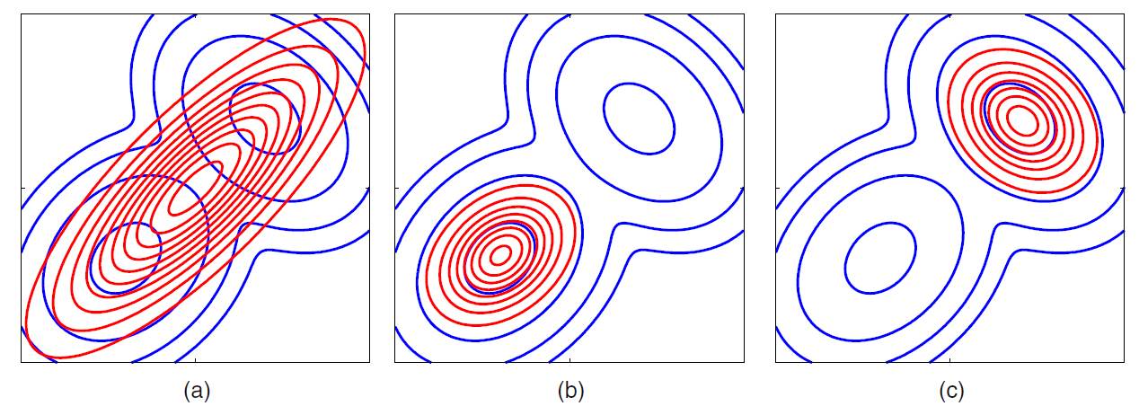
(a) : \(KL(p\mid \mid q)\) ( reverse KL )

(b) : \(KL(q\mid \mid p)\) (1)

(c) : \(KL(q\mid \mid p)\) (2)

• minimizing (a) : minimized by \(q(Z)\) that are nonzero, where \(p(Z)\) is non-zero
  • will average across all of the modes
  • lead to poor predictive distn
• minimizing (b,c) : minimized by \(q(Z)\) that avoid where \(p(Z)\) is small
  • will tent to find one of these multi-modes

both (a) and (b,c) are members of “alpha family”

\(\mathrm{D}_{\alpha}(p \| q)=\frac{4}{1-\alpha^{2}}\left(1-\int p(x)^{(1+\alpha) / 2} q(x)^{(1-\alpha) / 2} \mathrm{~d} x\right)\).

• when \(\alpha=0\) : symmetric divergence

  called “Helinger distance”

  \(\mathrm{D}_{\mathrm{H}}(p \| q)=\int\left(p(x)^{1 / 2}-q(x)^{1 / 2}\right) \mathrm{d} x\).

10-1-3. Ex) Univariate Gaussian

Factorized Variational approximation using Gaussian

Goal : infer posterior for

• mean \(\mu\)
• precision \(\tau\)

Likelihood : \(p(\mathcal{D} \mid \mu, \tau)=\left(\frac{\tau}{2 \pi}\right)^{N / 2} \exp \left\{-\frac{\tau}{2} \sum_{n=1}^{N}\left(x_{n}-\mu\right)^{2}\right\}\).

Conjugate prior ( Gaussian-Gamma conjuagte prior distn )

• mean (=Normal) : \(p(\mu \mid \tau) =\mathcal{N}\left(\mu \mid \mu_{0},\left(\lambda_{0} \tau\right)^{-1}\right)\)
• precision (=Gamma) : \(p(\tau) =\operatorname{Gam}\left(\tau \mid a_{0}, b_{0}\right)\)

We will consider a factorized variational approximation, as

\(q(\mu, \tau)=q_{\mu}(\mu) q_{\tau}(\tau)\).

( as we have found in \(\ln q_{j}^{\star}\left(\mathbf{Z}_{j}\right)=\mathbb{E}_{i \neq j}[\ln p(\mathbf{X}, \mathbf{Z})]+\text { const. }\)…. )

Mean (\(\mu\))

\(\begin{aligned} \ln q_{\mu}^{\star}(\mu) &=\mathbb{E}_{\tau}[\ln p(\mathcal{D} \mid \mu, \tau)+\ln p(\mu \mid \tau)]+\text { const } \\ &=-\frac{\mathbb{E}[\tau]}{2}\left\{\lambda_{0}\left(\mu-\mu_{0}\right)^{2}+\sum_{n=1}^{N}\left(x_{n}-\mu\right)^{2}\right\}+\text { const. } \end{aligned}\).

Thus \(q_{\mu}(\mu)\) follows \(\mathcal{N}\left(\mu \mid \mu_{N}, \lambda_{N}^{-1}\right)\)

• mean ) \(\mu_{N} =\frac{\lambda_{0} \mu_{0}+N \bar{x}}{\lambda_{0}+N}\)
• precision ) \(\lambda_{N} =\left(\lambda_{0}+N\right) \mathbb{E}[\tau]\)

for \(N \rightarrow \infty\)

• same as MLE result! (ignores prior, considers only data)

Precision (\(\tau\))

\(\begin{aligned} \ln q_{\tau}^{\star}(\tau)=& \mathbb{E}_{\mu}[\ln p(\mathcal{D} \mid \mu, \tau)+\ln p(\mu \mid \tau)]+\ln p(\tau)+\text { const } \\ =&\left(a_{0}-1\right) \ln \tau-b_{0} \tau+\frac{N}{2} \ln \tau \\ &-\frac{\tau}{2} \mathbb{E}_{\mu}\left[\sum_{n=1}^{N}\left(x_{n}-\mu\right)^{2}+\lambda_{0}\left(\mu-\mu_{0}\right)^{2}\right]+\text { const } \end{aligned}\).

Thus \(q_{\tau}(\tau)\) follows \(\operatorname{Gam}\left(\tau \mid a_{N}, b_{N}\right)\)

• \[a_{N}=a_{0}+\frac{N}{2}\]
• \[b_{N}=b_{0}+\frac{1}{2} \mathbb{E}_{\mu}\left[\sum_{n=1}^{N}\left(x_{n}-\mu\right)^{2}+\lambda_{0}\left(\mu-\mu_{0}\right)^{2}\right]\]

for \(N \rightarrow \infty\)

• same as MLE result! (ignores prior, considers only data)

Summary

• (step 1) make initial guess for \(\mathbb{E}[\tau]\)
• (step 2) re-compute \(q_{\mu}(\mu)\)
• (step 3) with revised distn, calculate \(\mathbb{E}[\mu]\) and \(\mathbb{E}\left[\mu^{2}\right]\)
• (step 4) re-compute \(q_{\tau}(\tau)\)

Repeat step1~step4 until convergence!

10-2. Illustration : Variational Mixture of Gaussian

\(p(\mathbf{Z} \mid \pi)=\prod_{n=1}^{N} \prod_{k=1}^{K} \pi_{k}^{z_{n k}}\).

\(p(\mathbf{X} \mid \mathbf{Z}, \boldsymbol{\mu}, \boldsymbol{\Lambda})=\prod_{n=1}^{N} \prod_{k=1}^{K} \mathcal{N}\left(\mathbf{x}_{n} \mid \boldsymbol{\mu}_{k}, \boldsymbol{\Lambda}_{k}^{-1}\right)^{z_{n k}}\).

priors for \(\mu, \Lambda\) and \(\pi\)

• \(\pi\) : \(p(\pi)=\operatorname{Dir}\left(\pi \mid \alpha_{0}\right)=C\left(\alpha_{0}\right) \prod_{k=1}^{K} \pi_{k}^{\alpha_{0}-1}\).

  • \(C\left(\alpha_{0}\right)\) is a normalizing constant

  • \(\alpha_0\) : effective prior number of observations

    ( if \(\alpha_0\) is small \(\rightarrow\) more effect on data )

• \(\mu\), \(\Lambda\) :

  \(\begin{aligned} p(\mu, \Lambda) &=p(\mu \mid \Lambda) p(\Lambda) \\ &=\prod_{k=1}^{K} \mathcal{N}\left(\mu_{k} \mid \mathbf{m}_{0},\left(\beta_{0} \Lambda_{k}\right)^{-1}\right) \mathcal{W}\left(\Lambda_{k} \mid \mathbf{W}_{0}, \nu_{0}\right) \end{aligned}\).

  • Gaussian-Wishart prior

    ( represents conjugate prior, when both mean and precision are unknown )

10-2-1. Variational Distribution

joint pdf : \(p(\mathbf{X}, \mathbf{Z}, \boldsymbol{\pi}, \boldsymbol{\mu}, \boldsymbol{\Lambda})=p(\mathbf{X} \mid \mathbf{Z}, \boldsymbol{\mu}, \boldsymbol{\Lambda}) p(\mathbf{Z} \mid \pi) p(\boldsymbol{\pi}) p(\boldsymbol{\mu} \mid \boldsymbol{\Lambda}) p(\boldsymbol{\Lambda})\)

variational distn : \(q(\mathbf{Z}, \boldsymbol{\pi}, \boldsymbol{\mu}, \boldsymbol{\Lambda})=q(\mathbf{Z}) q(\boldsymbol{\pi}, \boldsymbol{\mu}, \boldsymbol{\Lambda})\)

Sequential update can be easily done!

( as we have found in \(\ln q_{j}^{\star}\left(\mathbf{Z}_{j}\right)=\mathbb{E}_{i \neq j}[\ln p(\mathbf{X}, \mathbf{Z})]+\text { const. }\)…. )

• update \(q(\mathbf{Z})\)
• update \(q(\boldsymbol{\pi}, \boldsymbol{\mu}, \boldsymbol{\Lambda})\)

update \(q(\mathbf{Z})\)

\(\ln q^{\star}(\mathbf{Z})=\mathbb{E}_{\pi, \mu, \Lambda}[\ln p(\mathbf{X}, \mathbf{Z}, \boldsymbol{\pi}, \boldsymbol{\mu}, \boldsymbol{\Lambda})]+\text { const. }\).

\(\ln q^{\star}(\mathbf{Z})=\mathbb{E}_{\pi}[\ln p(\mathbf{Z} \mid \pi)]+\mathbb{E}_{\mu, \Lambda}[\ln p(\mathbf{X} \mid \mathbf{Z}, \boldsymbol{\mu}, \boldsymbol{\Lambda})]+\text { const. }\) ( by decomposing \(p(\mathbf{X}, \mathbf{Z}, \boldsymbol{\pi}, \boldsymbol{\mu}, \boldsymbol{\Lambda}))\)

\(\ln q^{\star}(\mathbf{Z})=\sum_{n=1}^{N} \sum_{k=1}^{K} z_{n k} \ln \rho_{n k}+\operatorname{const}\).

• where \(\begin{aligned} \ln \rho_{n k}=& \mathbb{E}\left[\ln \pi_{k}\right]+\frac{1}{2} \mathbb{E}\left[\ln \left|\boldsymbol{\Lambda}_{k}\right|\right]-\frac{D}{2} \ln (2 \pi) -\frac{1}{2} \mathbb{E}_{\boldsymbol{\mu}_{k}, \boldsymbol{\Lambda}_{k}}\left[\left(\mathbf{x}_{n}-\boldsymbol{\mu}_{k}\right)^{\mathrm{T}} \boldsymbol{\Lambda}_{k}\left(\mathbf{x}_{n}-\boldsymbol{\mu}_{k}\right)\right] \end{aligned}\)

\(q^{\star}(\mathbf{Z}) \propto \prod_{n=1}^{N} \prod_{k=1}^{K} \rho_{n k}^{z_{n k}}\) ( by taking exponential )

\(q^{\star}(\mathbf{Z})=\prod_{n=1}^{N} \prod_{k=1}^{K} r_{n k}^{z_{n k}}\) ( by normalizing )

• where \(r_{n k}=\frac{\rho_{n k}}{\sum_{j=1}^{K} \rho_{n j}}\)

optimal solution for the factor \(q(Z)\) takes the same functional form as the prior $$p(Z

\pi)$$

( since we have used conjugate prior! )

Result : \(\mathbb{E}\left[z_{n k}\right]=r_{n k}\)

update \(q(\boldsymbol{\pi}, \boldsymbol{\mu}, \boldsymbol{\Lambda})\)

\(\begin{array}{l} \ln q^{\star}(\pi, \mu, \Lambda)=\ln p(\pi)+\sum_{k=1}^{K} \ln p\left(\mu_{k}, \Lambda_{k}\right)+\mathbb{E}_{\mathbf{Z}}[\ln p(\mathbf{Z} \mid \pi)] +\sum_{k=1}^{K} \sum_{n=1}^{N} \mathbb{E}\left[z_{n k}\right] \ln \mathcal{N}\left(\mathbf{x}_{n} \mid \mu_{k}, \Lambda_{k}^{-1}\right)+\text {const. } \end{array}\).

• because \(q(\boldsymbol{\pi}, \boldsymbol{\mu}, \boldsymbol{\Lambda})=q(\boldsymbol{\pi}) \prod_{k=1}^{K} q\left(\boldsymbol{\mu}_{k}, \boldsymbol{\Lambda}_{k}\right)\)

\(q(\boldsymbol{\pi})\) : Dirichlet

• \(\ln q^{*}(\pi)=\left(\alpha_{0}-1\right) \sum_{k=1}^{K} \ln \pi_{k}+\sum_{k=1}^{K} \sum_{n=1}^{N} r_{n k} \ln \pi_{k}+\text { const }\).
• \(q^{\star}(\pi)=\operatorname{Dir}(\pi \mid \alpha)\).
  • where \(\alpha_{k}=\alpha_{0}+N_{k}\)

\(q\left(\boldsymbol{\mu}_{k}, \boldsymbol{\Lambda}_{k}\right)\) : Gaussian-Wishart

• \(q^{\star}\left(\boldsymbol{\mu}_{k}, \boldsymbol{\Lambda}_{k}\right)=\mathcal{N}\left(\boldsymbol{\mu}_{k} \mid \mathbf{m}_{k},\left(\beta_{k} \boldsymbol{\Lambda}_{k}\right)^{-1}\right) \mathcal{W}\left(\boldsymbol{\Lambda}_{k} \mid \mathbf{W}_{k}, \nu_{k}\right)\).

• where

  \(\begin{aligned} \beta_{k} &=\beta_{0}+N_{k} \\ \mathrm{~m}_{k} &=\frac{1}{\beta_{k}}\left(\beta_{0} \mathrm{~m}_{0}+N_{k} \overline{\mathrm{x}}_{k}\right) \\ \mathrm{W}_{k}^{-1} &=\mathrm{W}_{0}^{-1}+N_{k} \mathrm{~S}_{k}+\frac{\beta_{0} N_{k}}{\beta_{0}+N_{k}}\left(\overline{\mathrm{x}}_{k}-\mathrm{m}_{0}\right)\left(\overline{\mathrm{x}}_{k}-\mathrm{m}_{0}\right)^{\mathrm{T}} \\ \nu_{k} &=\nu_{0}+N_{k} \end{aligned}\).

These updating equations are analogous to “M-step”