[reliable] (paper 1) On Calibration of Modern Neural Networks

On Calibration of Modern Neural Networks

Contents

1. Abstract
2. Introduction
3. Definition
   1. Reliability Diagrams
   2. Expected Calibration Error (ECE)
   3. Maximum Calibration Error (MCE)
   4. Negative Log Likelihood (NLL)
4. Observing Miscalibration
   1. Model Capacity
   2. Batch Normalization (BN)
   3. Weight decay
   4. NLL
5. Calibration Methods
   1. Binary case
   2. Multi-class case

0. Abstract

NN은 poorly calibrated!

Calibration : “모델의 출력값이 실제 confidence (calibrated confidence) 를 반영하도록 만드는 과정”

• ex) classifier의 output이 0.8이라면, 80%의 확률로 해당 class이게끔 만드는 것!

1. Introduction

좋은 모델은

• 1) 성능 GOOD ( 성능 = accuracy )뿐만 아니라
• 2) 언제 맞을 지/틀릴 지 잘 알아야 한다

2)를 잘 하기 위해, prediction 뿐만 아니라 “calibrated confidence” measure 또한 제공해야!

( ex) calibrated confidence가 0.6이다 = 10번중 6번은 실제로 해당 class 여야 한다! )

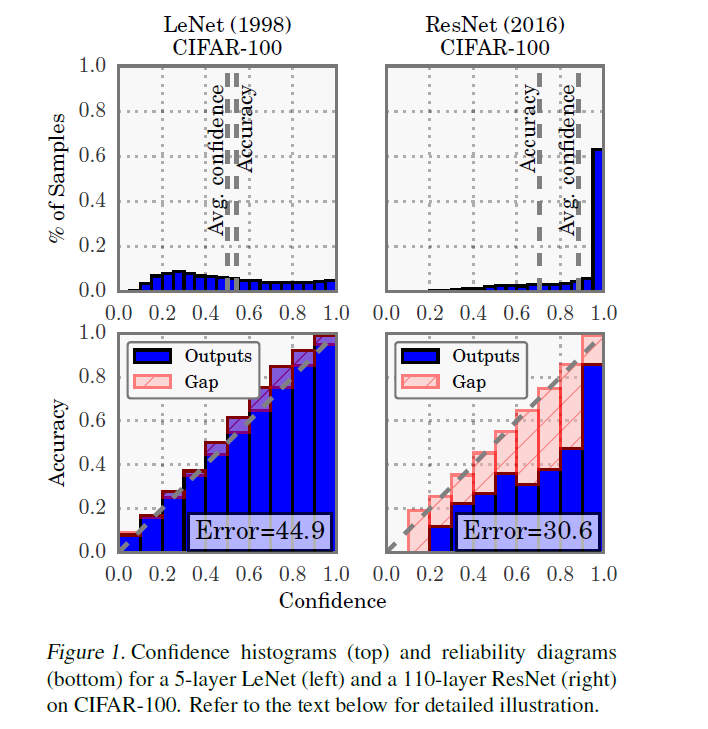
Example ) LeNet vs ResNet

결론 요약 :

• LeNet : 성능 soso, Calibration good
• ResNet : 성능 good, Calibration soso

• (TOP) prediction confidence의 분포

  ( = 즉, \(\hat{y}\)들의 분포 histogram으로 보면 된다 )

  • LeNet은 확신있게 답을 못하지만, ResNet은 근자감!

    ( LeNet의 경우, average confidence \(\approx\) accuracy )

    ( ResNet의 경우, average confidence \(>\) accuracy )

  • LeNet은 well-callibrated!

• (BOTTOM) Reliability Diagrams

  • 뒤에서 자세히 설명

이 논문의 목표는, NN이 miscalibrated된 것을 이해하는 것을 넘어서서, 어떻게 이를 해결할 지를 제안!

2. Definitions

NN으로 Multi-class classification하는 상황을 가정한다.

[ Notation 정리]

• \(X \in \mathcal{X}\) : input

• \(Y \in \mathcal{Y}=\{1, \ldots, K\}\) : output

  ( input과 output은 \(\pi(X, Y)=\) \(\pi(Y \mid X) \pi(X)\)를 따름 )

• \(h(X)=(\hat{Y}, \hat{P})\) : Neural Network

  • \(\hat{Y}\) : class prediction

  • \(\hat{P}\) : associated confidence ( = probability of correctness )

    ( 즉, \(\hat{P}=0.8\) 이다 = 10번 중 8번은 실제로 해당 class다! )

• Perfect Calibration

  = \(\mathbb{P}(\hat{Y}=Y \mid \hat{P}=p)=p, \quad \forall p \in[0,1]\)

2-1. Reliability Diagrams

“visual representation of model calibration”

• X축 : confidence
• Y축 : expected sample accuracy
• BEST 상황 : \(y=x\)

expected sample accuracy 계산 방법?

• 1) \(M\) 개의 interval bin으로 나눔

  ( ex. \(B_1\) : confidence가 0.0~0.1 …. \(B_{10}\) : confidence가 0.9~1.0 )

• 2) (\(M\)개 bin의) accuracy를 각각 구함

  \(\operatorname{acc}\left(B_{m}\right)=\frac{1}{ \mid B_{m} \mid } \sum_{i \in B_{m}} \mathbf{1}\left(\hat{y}_{i}=y_{i}\right)\).

• 3) (\(M\)개 bin의) average confidence를 각각 구함

  \(\operatorname{conf}\left(B_{m}\right)=\frac{1}{ \mid B_{m} \mid } \sum_{i \in B_{m}} \hat{p}_{i}\).

  ( \(\hat{p}_i\) : sample \(i\)의 confidence )

PERFECT case : \(\operatorname{acc}\left(B_{m}\right)=\operatorname{conf}\left(B_{m}\right)\)

2-2. Expected Calibration Error (ECE)

( scalar값으로 summary )

( ECE를 calibration을 측정하기 위한 primary empirical metric으로 사용 )

KEY : E [ confidence & accuracy사이의 차이 ]

• \(\underset{\hat{P}}{\mathbb{E}}[ \mid \mathbb{P}(\hat{Y}=Y \mid \hat{P}=p)-p \mid ]\).

마찬가지로, \(M\)개의 interval bin으로 나누고,

weighted average of bins’ accuracy / confidence difference

\(\mathrm{ECE}=\sum_{m=1}^{M} \frac{ \mid B_{m} \mid }{n} \mid \operatorname{acc}\left(B_{m}\right)-\operatorname{conf}\left(B_{m}\right) \mid\).

acc와 conf의 차이를 “calibration gap”이라고 부름

( ex. 위 Figure1의 아래 그림의 red 줄무늬 bar )

2-3. Maximum Calibration Error (MCE)

key idea : HIGH RISK에 더 높은 가중치 부여!

즉, 최악의 상황을 피하는데에 focus

• \(\max _{p \in[0,1]} \mid \mathbb{P}(\hat{Y}=Y \mid \hat{P}=p)-p \mid\).

\(\mathrm{MCE}=\max _{m \in\{1, \ldots, M\}} \mid \operatorname{acc}\left(B_{m}\right)-\operatorname{conf}\left(B_{m}\right) \mid .\).

ECE와 마찬가지로, MCE도 reliability diagram에 그릴 수 있다.

( ex. 위 Figure1의 아래 그림의 red 줄무늬 bar 중, 가장 긴 막대! ECE는 막대들 길이의 평균 )

2-4. Negative Log Likelihood (NLL)

( simple하니 설명 생략 )

\(\mathcal{L}=-\sum_{i=1}^{n} \log \left(\hat{\pi}\left(y_{i} \mid \mathbf{x}_{i}\right)\right)\).

3. Observing Miscalibration

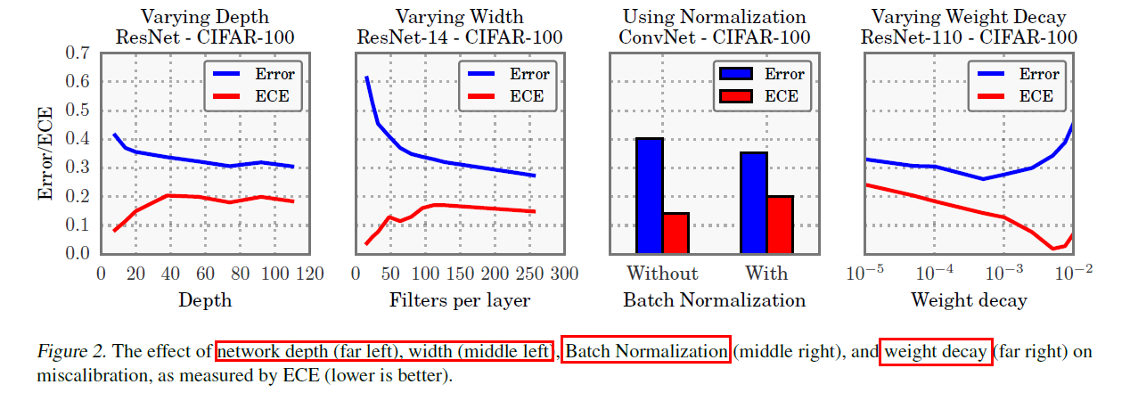
model capacity의 향상 & lack of regularization \(\rightarrow\) “model miscalibration”

3-1. Model Capacity

• 요즈음 갈 수록 model capacity 엄청 향상!
• 하지만, 이에 따라 model miscalibration야기!

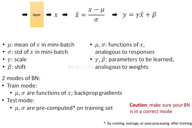
3-2. Batch Normalization (BN)

• minimize distribution shifts in activation function
• 하지만, 이에 따라 model miscalibration야기!

3-3. Weight decay

• NN에서 overfitting 방지하기 위한 regularization 방법

• 하지만 BN 등장 이후, L2-reg 없는게 오히려 더 generalize 잘 하는 경향!

  ( 요즈음은 쓴다 해도 매우 작은 값으로 사용 )

• 하지만, weight decay 적게 쓸 수록 calibration에 악영향!

3-1~ 3-3을 요약한 실험

3-4. NLL

model calibration을 indirectly 측정하기 위해 NLL 사용

“NLL과 accuracy의 차이”를 통해 miscalibration의 정도를 파악!

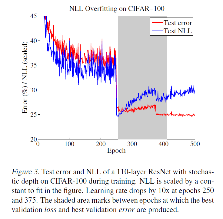
놀라운 점 !! NLL을 objective function으로 삼고 과적합해도 accuracy에는 오히려 GOOD!

4. Calibration Methods

4-1. Binary case

a) Histogram Binning

• 간단한 non-parametric 방법

• uncalibrated prediction \(\hat{p}_i\)를 \(M\)개의 bin으로 나눔

  ( 각 bin을 대표하는 calibrated score \(\theta_m\) 이 존재 )

• ex) 만약 \(\hat{p}_{729}\) 가 \(B_7\)에 배정되었으면, \(\hat{p}_{729}\)의 calibrated score는 \(\theta_7\)

• 특정 test data의 예측값이 어떤 \(B_k\)에 떨어지게 되면, 해당 test data의 calibrated score는 \(\theta_k\)로 예측된다

• Loss Function :

  \(\min _{\theta_{1}, \ldots, \theta_{M}} \sum_{m=1}^{M} \sum_{i=1}^{n} 1\left(a_{m} \leq \widehat{p}_{i}<a_{m+1}\right)\left(\theta_{m}-y_{i}\right)^{2}\).

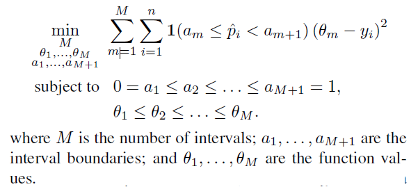
b) Isotonic regression

• most common non-parametric 방법

• piecewise constant function \(f\)를 학습

  ( \(\widehat{q}_{i}=f\left(\widehat{p}_{i}\right)\) )

• Loss Function : \(\sum_{i=1}^{n}\left(f\left(\widehat{p}_{i}\right)-y_{i}\right)^{2}\)

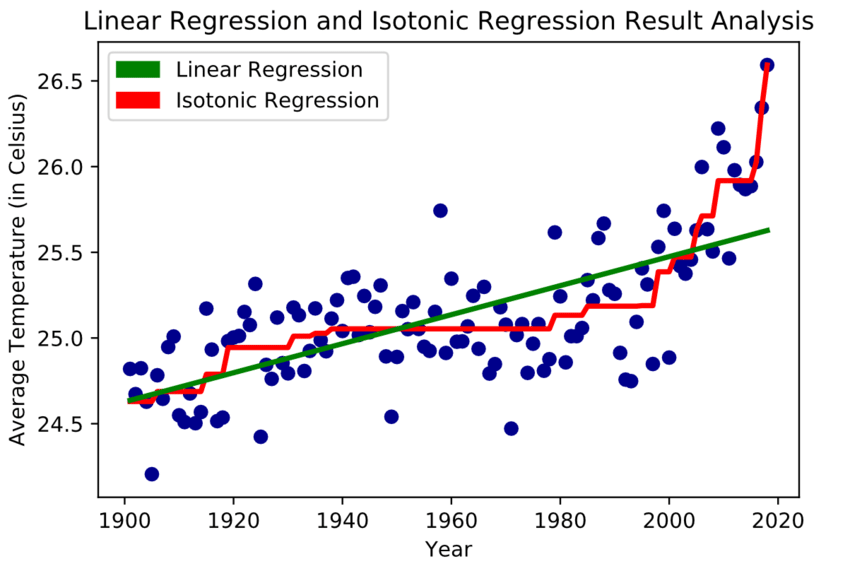
다만, 여기서 \(f\)가 “piecewise” function이기 때문에, 위 loss function을 optimize하는 것은 곧 아래와 같다.

c) Bayesian Binning into Quantiles (BBQ)

• histogram binning의 extension ( Bayesian model averaging을 사용하여 )

• 식을 통해 직관적으로 이해!

  \(\begin{aligned} \mathbb{P}\left(\hat{q}_{t e} \mid \hat{p}_{t e}, D\right) &=\sum_{s \in S} \mathbb{P}\left(\hat{p}_{t e}, S=s \mid \hat{p}_{t e}, D\right) \\ &=\sum_{s \in S} \mathbb{P}\left(\hat{q}_{t e} \mid \hat{p}_{t e}, S=s, D\right) \mathbb{P}(S=s \mid D) \end{aligned}\).

  ( 하나의 bin에 귀속시키는 것이 아니라, 여러 bin에 soft하게 귀속된다고 보면 됨! )

• weight는 아래와 같이 구함 (\(\sum=1\) )

  \(\mathbb{P}(S=s \mid D)=\frac{\mathbb{P}(D \mid S=s)}{\sum_{s^{\prime} \in S} \mathbb{P}\left(D \mid S=s^{\prime}\right)}\).

d) Platt scaling

• parametric한 방법

• 아래 식의 scalar parameter \(a\)와 \(b\)를 학습

  calibrated probability : \(\hat{q}_{i}=\sigma\left(a z_{i}+b\right)\).

  ( validation dataset의 NLL minimize학습하도록 \(a\)와 \(b\)를 설정 )

  여기서 \(z_i\)는 network의 ouput인 logit 형태

4-2. Multi-class case

( 이제 network logit인 \(z_i\)는 vector! )

• \(\hat{y}_{i}=\operatorname{argmax}_{k} z_{i}^{(k)}\).

• \(\hat{p}_{i}=\max _{k} \sigma_{\mathrm{SM}}\left(\mathbf{z}_{i}\right)^{(k)}\),

  where \(\sigma_{\mathrm{SM}}\left(\mathbf{z}_{i}\right)^{(k)}=\frac{\exp \left(z_{i}^{(k)}\right)}{\sum_{j=1}^{K} \exp \left(z_{i}^{(j)}\right)}\)

a) Extension of binning methods

아까는 binary했으니까 0~1사이의 bin으로 가능했었음. 이제는 multi-class (\(K>2\))

\(K\)개의 one-vs-ALL 문제로써 생각!

b) Matrix and vector scaling

Platt scaling의 multi-class 버전으로 생각하면 됨!

\(\begin{array}{l} \hat{q}_{i}=\max _{k} \sigma_{\mathrm{SM}}\left(\mathbf{W} \mathbf{z}_{i}+\mathbf{b}\right)^{(k)} \\ \hat{y}_{i}^{\prime}=\underset{k}{\operatorname{argmax}}\left(\mathbf{W} \mathbf{z}_{i}+\mathbf{b}\right)^{(k)} . \end{array}\).

c) Temperature Scaling

Platt scaling의 “간단한” multi-class 버전으로 생각하면 됨!

모든 class에 대해서 하나의 scalar parameter \(T\)를 사용!

\(\hat{q}_{i}=\max _{k} \sigma_{\mathrm{SM}}\left(\mathbf{z}_{i} / T\right)^{(k)}\).

• 여기서 \(T\)를 temperature라고 부름

  ( \(T>1\)일 경우, softmax를 soften한다! )

• \(T\rightarrow \infty\) : \(\hat{q}_{i}= \frac{1}{K}\) ( 예측값 : 정말 아무것도 모르겠어~ )

• \(T\rightarrow 0\) : \(\hat{q}_{i}= 1\) ( 예측값 : 근자감 )

\(T\)도 validation dataset을 통해 최적으로 tuning해서 사용함

주로 사용 분야 :

• knowledge distillation