30.Actor-Critic ( 가치 기반 + Policy Gradient )

( 참고 : Fastcampus 강의 )

[ 30. Actor-Critic ( 가치 기반 + Policy Gradient ) ]

Contents

1. REINFORCE vs Actor-Critic
   1. REINFORCE
   2. Actor Critic
2. Q Actor-Critic
3. Variance Reduction ( via Baseline )
   1. Baseline : \(V^{\pi}(s)\)
   2. Advantage Function
   3. Advantage Function 구현 1
   4. Advantage Function 구현 2
4. 다양한 Policy Gradient 알고리즘들

1. REINFORCE vs Actor-Critic

우리는 policy의 gradient를 아래와 같이 구했었다.

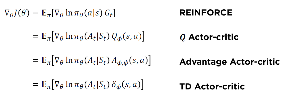
\(\begin{aligned} \nabla_{\theta} J(\theta) &=\mathbb{E}_{\pi}\left[\nabla_{\theta} \ln \pi_{\theta}(a \mid s) Q^{\pi}(s, a)\right] \\ &=\mathbb{E}_{\pi}\left[\nabla_{\theta} \ln \pi_{\theta}\left(A_{t} \mid S_{t}\right) G_{t}\right] \end{aligned}\).

(1) REINFORCE

위 \(\nabla_{\theta} J(\theta)\) 에서, \(G_t\)는 아래와 같이 계산되었었고,

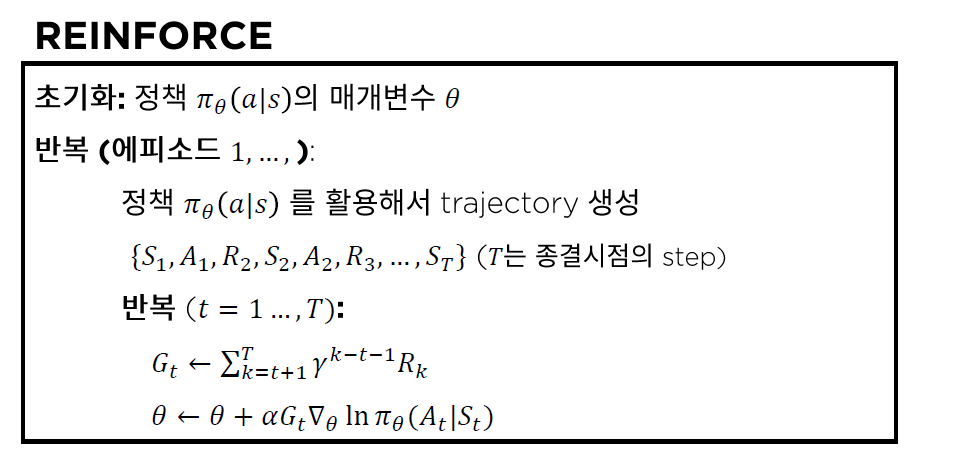
• \(G_{t} \leftarrow \sum_{k=t+1}^{T} \gamma^{k-t-1} R_{k}\),

따라서 \(\theta\)에 대한 updating equation은 아래와 같았었다.

• \(\theta \leftarrow \theta+\alpha G_{t} \nabla_{\theta} \ln \pi_{\theta}\left(A_{t} \mid S_{t}\right)\).
  

하지만 위 방법에 문제점이 있었다. Return인 \(G_t\)가 unbiased estimator이긴 하지만, variance가 크다는 문제점이 있었다 (\(\because\) Monte Carlo 방법)

(2) Actor-Critic

위의 문제를 어떻게 해결할까 하다가 나온 것이 바로 Actor Critic이다.

Actor Critic은, 위의 \(G_t\)를 학습을 통해서 배워보면 어떨까라는 관점에서 시작되었다.

[ key point ]

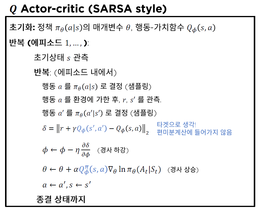
​ “학습된” 행동 가치 함수 (action-value function)인 \(Q_{\phi}^{\pi}(s, a)\)를 \(G_t\) 대신 사용하자!

• \(G_{t} \leftarrow Q_{\phi}^{\pi}\left(S_{t}, A_{t}\right)\).
• \(\theta \leftarrow \theta+\alpha \gamma^{t} G_{t} \nabla_{\theta} \ln \pi_{\theta}\left(A_{t} \mid S_{t}\right)\).
  

이름이 왜 Actor-critic ?

• actor가 상황(state)를 보고 행동(action)을 하고 …………. \(\pi_{\theta}(a \mid s)\)
• critic이 상황(state)과 actor의 행동(action)을 보고 감독(평가)를 함으로써, 보다 나은 행동을 하도록 만든다 …………. \(Q_{\phi}^{\pi}(s, a)\)

2. Q Actor-Critic

(revisit) REINFORCE

REINFORCE 알고리즘은 아래와 같다.

3. Variance Reduction ( via Baseline )

(1) Baseline : \(V^{\pi}(s)\)

REINFORCE 때에도 배웠지만, 우리는 gradient의 variance를 줄이기 위해 baseline을 빼줬었다.

이를 Actor-Critic에도 적용하자면, 아래와 같다.

\(\nabla_{\theta} J(\theta) \propto \sum_{s} d^{\pi}(s) \sum_{a \in \mathcal{A}} \nabla_{\theta} \pi_{\theta}(a \mid s)\left(Q^{\pi}(s, a)-b(s)\right)\).

• 여기서 \(b(s)\)는, \(a\) 와 무관한 이상, 그 어떠한 것도 가능하다. 하지만 이에 대해 제일 자연스러운 선택은 주로 \(V^{\pi}(s)\)이다.

(2) Advantage Function

Baseline을 \(V^{\pi}(s)\)로 생각하여, 이를 빼준 부분 ( \(Q^{\pi}(s, a)-b(s)\) )을 Advantage Function이라고 부른다.

그 이유는, 위 식의 의미를 생각해보면 꽤 직관적이다.

Advantage function : \(A^{\pi}(s, a)=Q^{\pi}(s, a)-V^{\pi}(s)\)

• 의미 : 특정 상황 \(s\)에서, 행동 \(a\)가 다른 행동들에 비해 얼마나 (상대적으로) 좋은가?

위 방법을 구현하는데에는 크게 2가지 방법이 있다.

(3) Advantage Function 구현 1

\(A^{\pi}(s, a) \approx Q_{\phi}^{\pi}(s, a)-V_{\psi}^{\pi}(s)\).

• 행동 가치 함수(\(Q^{\pi}(s, a)\)) & 상태 가치 함수( \(V^{\pi}(s)\)) 모두 모델링
  • \(Q^{\pi}(s, a) \approx Q_{\phi}^{\pi}(s, a)\).
  • \(V^{\pi}(s) \approx V_{\psi}^{\pi}(s)\).
• policy gradient : \(\nabla_{\theta} J(\theta)=\mathbb{E}_{\pi}\left[\nabla_{\theta} \ln \pi_{\theta}(a \mid s) A^{\pi}(s, a)\right]\)
  

단점 :

• 3개의 서로 다른 모델 \(Q_{\phi}^{\pi}(s, a), V_{\psi}^{\pi}(s), \pi_{\theta}(a \mid s)\) 을 학습해야 한다.

(4) Advantage Function 구현 2

( 결론 : TD error 사용을 통해, 위의 (3)과 달리, 2개의 모델만을 학습해도 된다 )

\(A^{\pi}(s, a)=\mathbb{E}_{\pi}\left[\delta^{\pi} \mid s, a\right]\).

• (TRUE) TD error : \(\delta^{\pi}{=} r+V^{\pi}\left(s^{\prime}\right)-V^{\pi}(s)\)

• (TRUE) 행동 가치 함수 : \(Q^{\pi}(s, a)=\mathbb{E}_{\pi}\left[r+\gamma V^{\pi}\left(s^{\prime}\right) \mid S_{t}=s, A_{t}=a\right]\)

• [증명] (True) TD error 는 Advantage function 의 Unbiased Estimator

  \(\begin{aligned} \mathbb{E}_{\pi}\left[\delta^{\pi} \mid s, a\right] &=\mathbb{E}_{\pi}\left[r+V^{\pi}\left(s^{\prime}\right) \mid s, a\right]-V^{\pi}(s) \\ &=Q^{\pi}(s, a)-V^{\pi}(s) \\ &=A^{\pi}(s, a) \end{aligned}\).

• 하지만, True TD Error는 알기 어려우므로, 아래와 같이 모델링한다.

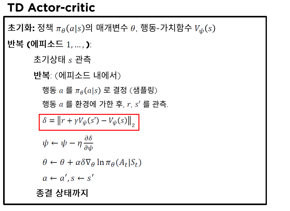
  • \(\delta_{\psi}=r+\gamma V_{\psi}^{\pi}\left(s^{\prime}\right)-V_{\psi}^{\pi}(s)\).
    

2개의 서로 다른 모델 \(V_{\psi}^{\pi}(s), \pi_{\theta}(a \mid s)\) 만 학습하면 된다!

TD Actor Critic

4. 다양한 Policy Gradient 알고리즘들