33.(paper 1) DQN (Deep Q-Network)

( 참고 : Fastcampus 강의 )

[ 33.(paper 1) DQN (Deep Q-Network) ]

Contents

1. Problems of RL
2. Non-stationary Target
3. Idea of DQN
4. DQN (Deep Q-Network)
   1. Replay Memory
   2. Fixed Q-target
   3. 기타
5. DQN Summary

간단 요약

• Sensory Data (이미지 데이터)를 통해 곧바로 정책을 학습 ( CNN 사용 )
• 심층신경망을 사용
• 각종 RL이 가지던 기존의 문제점들을 해결 ( 아래 참조 )
• [Key word] Experinece Replay, Target Network

1. Problems of RL

(1) sparse reward

• (일반적) DL : labeled training dataset을 통해 학습

• RL : 오로지 reward를 통해서만 학습되고, 심지어 reward도 sparse!

(2) iid assumption 불가

• 현재 state & 다음 state간의 correlation이 크다

(3) Non-stationary Target

• 예측하려는 대상 자체가 fixed 되어있지 않다

2. Non-stationary Target

우리의 타겟값(\(y\)) 조차 fixed된 값이 아니다!

최적의 action-value function을 근사하기 위한 loss function(MSE)를 적으면 아래와 같다.

• \(L_{i}\left(\theta_{i}\right)=\mathbb{E}_{s, a, r, s^{\prime}}\left[\left(r+\gamma \max _{a^{\prime}} Q\left(s^{\prime}, a^{\prime} ; \theta_{i}\right)-Q\left(s, a ; \theta_{i}\right)\right)^{2}\right]\).

즉, 근사하고자 하는 대상을 다시 적자면 아래와 같다.

• \(y_{i}=r+\gamma \max _{a^{\prime}} Q\left(s^{\prime}, a^{\prime} ; \theta_{i}\right)\).

위 식에서 알 수 있다시피, \(Q\left(s, a ; \theta_{i}\right)\) 가 \(Q\) 함수에 dependent하므로, \(Q\) 함수가 update됨에 따라 target 값 또한 계속 변화하는 상황이다.

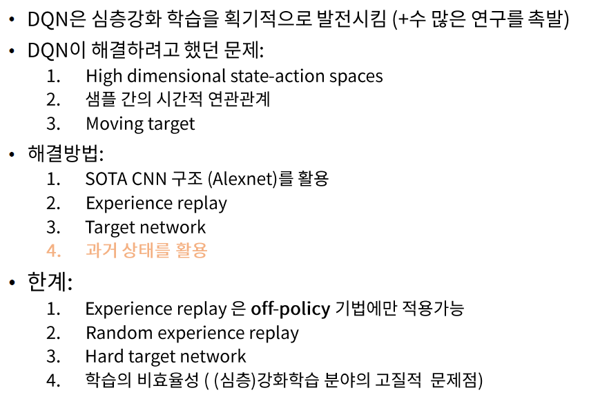
3. Idea of DQN

DQN은 위의 문제를, 아래와 같은 방법으로 해결한다.

Problem 1 : correlation between samples

\(\rightarrow\) Solution 1 : Experience Replay

Problem 2 : non-stationary target

\(\rightarrow\) Solution 2 : fixed Q-target

HOW?

• 1) raw pixel 그대로 input data로 사용 (전처리 X)
• 2) function approximator : CNN
• 3) 하나의 agent가 여러 종류의 Atari game을 학습하도록
• 4) Experience replay로 효율성 \(\uparrow\)

4. DQN (Deep Q-Network)

DQN의 Forward

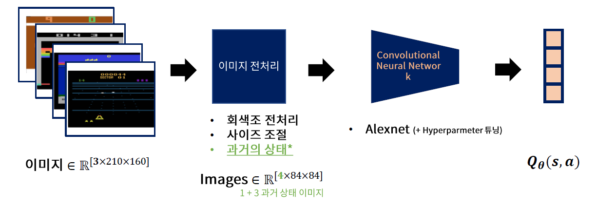
• 현재 상태 \(t\) 이전의 3 step (\(t-1,t-2,t-3\) )의 image를 함께 concatenate하여 forward한다
• feature extraction을 위해 사용하는 CNN 구조는 Alexnet
• Output : \(Q_{\theta}(s,a)\)

(1) Replay Memory ( Experinece Replay )

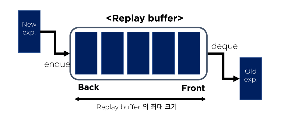
Replay Memory를 통해 correlation을 줄이기!

1. 기억 저장

   • agent의 경험 ( \(e_{t}=\left(s_{t}, a_{p}, r_{p}, s_{t+1}\right)\) )을 time step 단위로 \(D_{t}=\left\{e_{1}, \ldots, e_{t}\right\}\)에 저장

2. 학습 진행

   • 저장된 기억(=\(D_t\))으로부터 sampling 하여 구성된 mini-batch 통해 학습 진행 ( Batch Q-update )

     ( uniform sample : \((s, a, r, s) \sim U(D))\) )

   • mini-batch가 sequential 하지 않기 때문에, decorrelated

   • 과거 경험에 대한 반복학습 OK

   • (paper) replay memory size = 1,000,000

Batch Q-update

case 1) Online update

• \(Q(s, a) \leftarrow Q(s, a)+\eta\left(r+\gamma \max _{a^{\prime}} Q\left(s^{\prime}, a^{\prime}\right)-Q(s, a)\right)\).

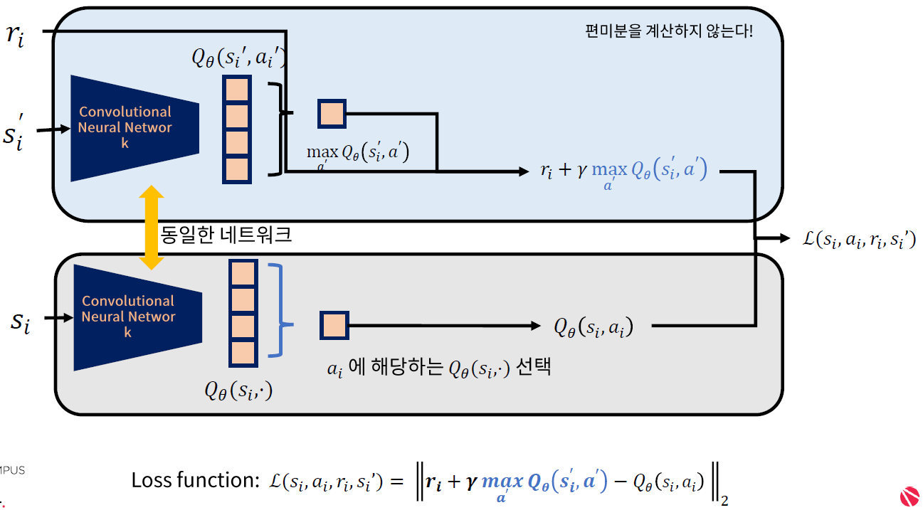
case 2) Function Approximation

• \(\theta \leftarrow \theta+\eta \frac{\partial \mathcal{L}\left(s, a, r, s^{\prime}\right)}{\partial \theta}\).
  • \(\mathcal{L}\left(s_{i}, a_{i}, r_{i}, s_{i}^{\prime}\right)=\left\|r_{i}+\gamma \max _{a} Q_{\theta}\left(s_{i}^{\prime}, a^{\prime}\right)-Q_{\theta}\left(s_{i}, a_{i}\right)\right\|_{2}\).

case 3) Function Approximation + Experience Replay

• \(\theta \leftarrow \theta+\eta \frac{\partial \frac{1}{m} \sum_{i=1}^{\mathrm{m}} \mathcal{L}\left(s_{i}, a_{i}, r_{i}, s_{i}^{\prime}\right)}{\partial \theta}\).

  • \(\mathcal{L}\left(s_{i}, a_{i}, r_{i}, s_{i}^{\prime}\right)=\left\|r_{i}+\gamma \max _{a} Q_{\theta}\left(s_{i}^{\prime}, a^{\prime}\right)-Q_{\theta}\left(s_{i}, a_{i}\right)\right\|_{2}\).

    where \(\left(s_{i}, a_{i}, r_{i}, s_{i}^{\prime}\right) \sim \mathcal{D}\).

위의 case 3)에서 정의한 loss function은, target - prediction 값의 L2 norm이다.

여기서 target은 계속 움직이게 되는데, 이를 고정시키기 위해 아래와 같은 방법론을 제안한다.

(2) Fixed Q-target ( Target Network )

\(Q(s, a ; \theta)\) 와 동일한 네트워크 구조를 가진 ( parameter는 다른 )

독립적인 TARGET network \(\hat{Q}\left(s, a ; \theta^{-}\right)\)생성

\(\rightarrow\) 이를 Q-learning target \(y_{i}\) 를 설정하는데에 이용한다.

\(y_{i} =r+\gamma \max _{a} \hat{Q}\left(s^{\prime}, a^{\prime} ; \theta_{i}^{-}\right) \\\).

\(\begin{aligned} L_{i}\left(\theta_{i}\right) &=\mathbb{E}_{(s, a, r s) \sim U(D)}\left[\left(y_i -Q\left(s, a ; \theta_{i}\right)\right)^{2}\right] \\ &=\mathbb{E}_{(s, a, r s) \sim U(D)}\left[\left(r+\gamma \operatorname{rmax}_{a} \hat{Q}\left(s^{\prime}, a^{\prime} ; \theta_{i}^{-}\right)-Q\left(s, a ; \theta_{i}\right)\right)^{2}\right] \end{aligned}\).

Target Network \(\hat{Q}\left(s, a ; \theta^{-}\right)\)의 parameter \(\theta^{-}\)는 “매 \(C\) step 마다”,

Q Network \(Q(s, a ; \theta)\)의 parameter \(\theta\)로 동일하게 update된다. ( paper : set \(C=10, 000\) )

(3) 기타

gradient exploration 방지 위해 gradient clipping 사용

5. DQN Summary

(1) 전반적인 Training 과정

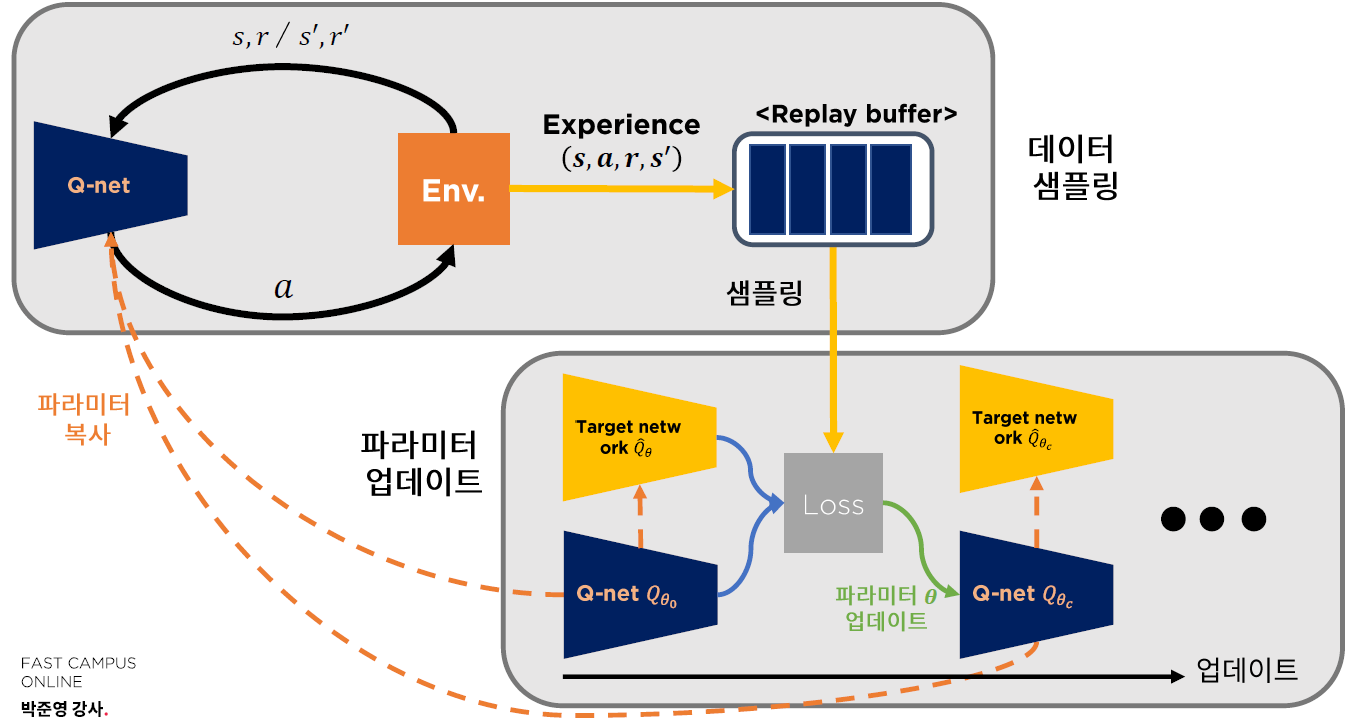
(2) Pseudocode

.

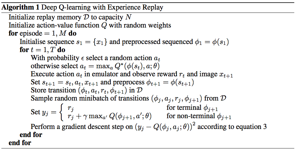(3) + \(\alpha\)

Hard Update ( = Hard Target update )

• Q-network의 파라미터를 ( 매 \(C\) step 마다) 그대로 복사 해서 Target Network를 생성한다

Soft Update ( = Soft Target Update )

• DDPG (Deep Deterministic Policy Gradient) 논문에서 제안

• \(\theta^{\prime} \leftarrow \tau \theta+(1-\tau) \theta^{\prime}\).

  위 식과 같이, 기존 & 새로운 parameter의 weighted average 형태로 update를한다

  • \(\tau = 0\) : 매 \(C\) step마다 hard update
  • \(\tau=1\) : 아예 update 안함

(4) Summary