36.(paper 2) DQN을 개선하기 위한 방법들

( 참고 : Fastcampus 강의 )

[ 36.(paper 2) DQN을 개선하기 위한 방법들 ]

DQN이 보다 잘 작동하도록 제안된 알고리즘들

• Double Q-Learning
• Prioritized Replay
• Dueling Replay
• Rainbow

1. Double Q-Learning (2010)

Double Q-Learning이 풀고자 하는 문제 : “Q-learning의 Maximization Bias”

• 가치함수를 실제보다 높게 평가하는 bias

  ( 즉, Q-Learner가 가치 함수 \(Q(s,a)\)를 실제 값 보다 높게 평가하는 bias )

1) Example of Maximization Bias

(1) Setting

• “state의 개수 = 1”인 MDP

• “action의 차원 = 2’

  \(\rightarrow\) \(\mathbb{E}\left(r \mid a_{1}\right)=\mathbb{E}\left(r \mid a_{2}\right)=0\)

(2) 과정

• 1) MDP로부터 unbiased estimator \(\hat{Q}\left(a_{1}\right), \hat{Q}\left(a_{2}\right)\) 를 구함
• 2) 이를 통해 최적의 Q-learning의 정책 \(\hat{\pi}=\underset{a}{\operatorname{argmax}} \hat{Q}(a)\) 를 찾음

(3) 결론

• \(V^{\widehat{\pi}}=\mathbb{E}_{\widehat{\pi}}\left[\max \left(\hat{Q}\left(a_{1}\right), \hat{Q}\left(a_{2}\right)\right)\right] \geq \max \left[\mathbb{E}_{\hat{\pi}}\left(\hat{Q}\left(a_{1}\right)\right), \mathbb{E}_{\hat{\pi}}\left(\hat{Q}\left(a_{2}\right)\right)\right]=\max [0,0]=0=V^{*}\).

\(\rightarrow\) \(Q\) -learning agent는 실제 가치함수 \(V^{*}\) 보다 높게 \(V^{\widehat{\pi}}\) 를 추산한다!

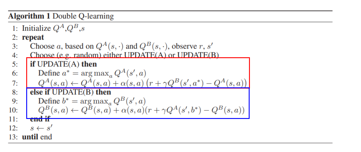
위 문제를 해결하기 위해 고안된 Double Q-Learning (2010)

2) Double Q-Learning

Key Idea : 2개의 Q-Learner를 학습함으로써 Maximization bias를 완화!

\(a^{*}=\operatorname{argmax}_{a} Q_{1}(s, a)\) 라고 하면, \(\mathbb{E}\left[Q_{2}\left(s, a^{*}\right)\right]=Q\left(s, a^{*}\right)\)

( \(\because\) \(Q_2\)는 \(Q\)의 unbiased estimator )

기타

• Double Q-Learning은 DQN이 나오기 전에 나온 것!
• 이를 적용한 Deep Double Q-Learning, Clipped Double Q-Learning이 나옴
  • Deep Double Q-Learning : \(Q_2\)를 target network로!
  • Clipped Double Q-Learning : \(Q_1,Q_2\) 중 낮은 값을 사용

2. Prioritized Replay

1) [Review] Prioritized Sweeping

• Bellman Error가 큰 \(s\) 부터 update

  \(\text { Bellman error }(s)= \mid \mid \max _{a \in \mathcal{A}}\left(R_{s}^{a}+\gamma \sum_{s^{\prime} \in \delta} P_{s S^{\prime}}^{a} V\left(s^{\prime}\right)\right)-V(s) \mid \mid\).

• Policy Evaluation, Value Iteration의 속도가 빨라짐

2) Prioritized Replay

Experience Replay를 할 때…

• Replay Memory에서 sampling 시 weight를 반영 하여 sampling한다

Sample (experiment)’s Weight

• \(p_{i} \propto \mid \mid r_{i}+\gamma \max _{a^{\prime}} Q_{\theta}\left(s_{i}^{\prime}, a^{\prime}\right)-Q_{\theta}\left(s_{i}, a_{i}\right) \mid \mid _{w}\).
  • \(r_{i}+\gamma \max _{a^{\prime}} Q_{\theta}\left(s_{i}^{\prime}, a^{\prime}\right)\) : target
  • \(Q_{\theta}\left(s_{i}, a_{i}\right)\) : prediction
• 직관적 해석 : Bellman error \(\uparrow\) \(\rightarrow\) Sampling 확률 \(\uparrow\)
• 당연히 normalization (with softmax)를 해줘야지

3. Dueling Network

( TD Actor Crictic에서 사용한 “Advantage Function” 복습 )

1) Advantage Function

[ \(Q,V,A\)의 관계 ]

\(Q^{\pi}(s, a)=V^{\pi}(s)+A^{\pi}(s, a)\).

• \(A^{\pi}(s, a)=Q^{\pi}(s, a)-V^{\pi}(s)\) .
• \(V^{\pi}(s)=Q^{\pi}(s, a)-A^{\pi}(s, a)\) .

\(V^{\pi}(s)=\mathbb{E}_{a \sim \pi(s)}\left[Q^{\pi}(s, a)\right]\).

• ( \(\because\) \(\mathbb{E}_{a \sim \pi(s)}\left[A^{\pi}(s, a)\right]=0\) )

Q-Learning에서 학습하는 action : \(a^{*}=\underset{a^{\prime} \in \mathcal{A}}{\operatorname{argmax}} Q\left(s, a^{\prime}\right)\).

Optimal Action에 대해서는 advantage=0이 된다. ( \(Q=V\))

• \(Q\left(s, a^{*}\right)=V(s) \rightarrow A\left(s, a^{*}\right)=0\).

2) Dueling Network

idea : \(Q\) 값을 \(V+A\) 꼴로 계산하기

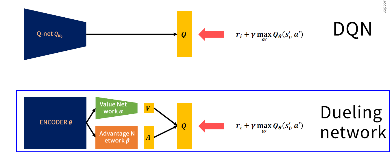
Estimate Q(s,a) with V(s), A(s,a)

\(Q(s, a ; \theta, \alpha, \beta)=V(s ; \theta, \beta)+A(s, a ; \theta, \alpha)\).

\(\rightarrow\) 문제점 : 두 합의 조합이 unique하지 않다!

# Case 1)

\(Q(s, a ; \theta, \alpha, \beta)=V(s ; \theta, \beta)+ \left(A(s, a ; \theta, \alpha)-\max _{a^{\prime}} A(s, a ; \theta, \alpha)\right) \\\).

• let \(\widetilde{A}\left(s, a^{*} ; \theta, \alpha\right)=\left(A(s, a ; \theta, \alpha)-\max _{a^{\prime}} A(s, a ; \theta, \alpha)\right)\)

• 만약 최적의 행동 \(a^{*}\)를 했을 때 ( \(a^{*}=\underset{a^{\prime} \in \mathcal{A}}{\operatorname{argmax}} Q\left(s, a^{\prime}\right)\) )

  • \(Q\left(s, a^{*} ; \theta, \alpha, \beta\right)=V(s ; \theta, \beta)\).
  • \(\widetilde{A}\left(s, a^{*} ; \theta, \alpha\right)=0\).

# Case 2)

( 위의 Case1의 argmax 부분 때문에 unstable한 학습 )

\(\begin{aligned} Q(s, a ; \theta, \alpha, \beta) &=V(s ; \theta, \beta)+\left(A(s, a ; \theta, \alpha)-\underset{a^{\prime}}{\mathbb{E}}\left[A\left(s, a^{\prime} ; \theta, \alpha\right)\right]\right) \end{aligned}\).

• let \(\widetilde{A}\left(s, a^{*} ; \theta, \alpha\right)=\left(A(s, a ; \theta, \alpha)-\underset{a^{\prime}}{\mathbb{E}}\left[A\left(s, a^{\prime} ; \theta, \alpha\right)\right]\right)\)
• 이론적으로 덜 타당해보여도, 실제로 Case 1보다 더 잘 작동함

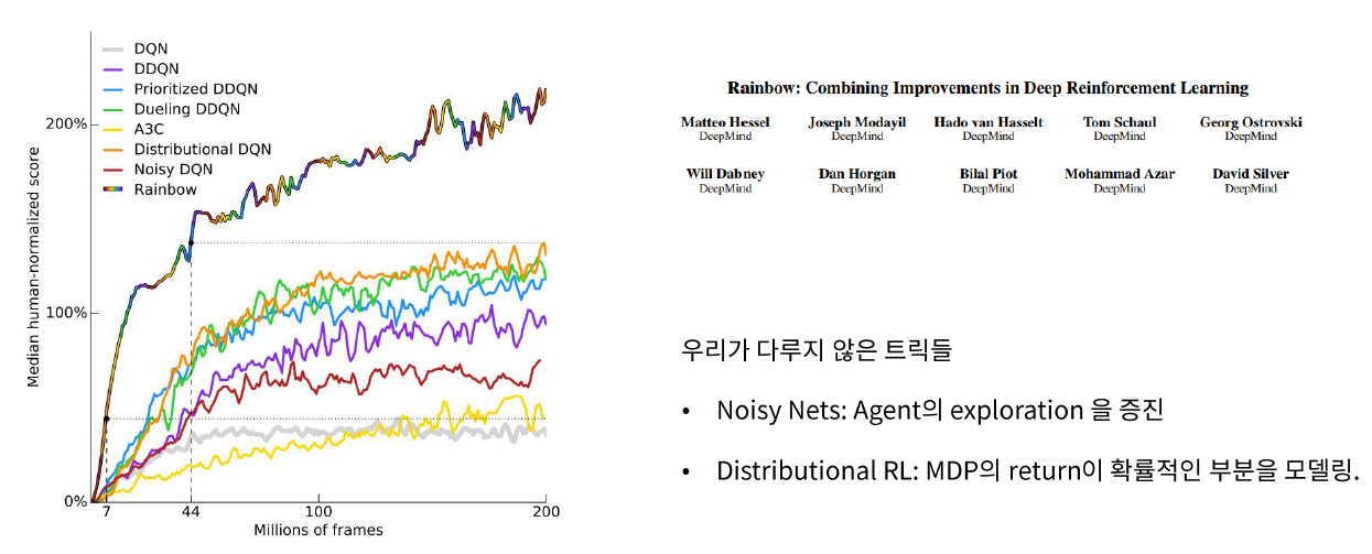
4. Rainbow

위의 모든 technique들을 다 합친 알고리즘