( 참고 : Fastcampus 강의 )
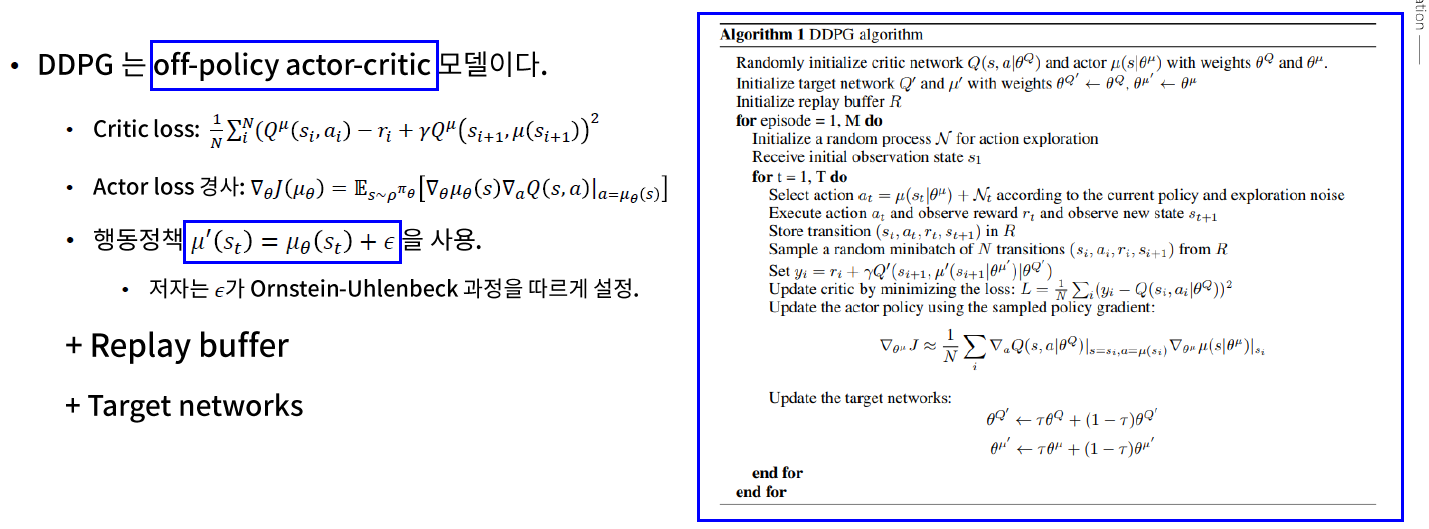
[ 37.(paper 3) DDPG (Deep Deterministic Policy Gradient) ]
1. Introduction
DDPG = (1) + (2)
- (1) DQN (Deep Q-Network)
- (2) DPG (Deterministic Policy Gradient)
Key Idea
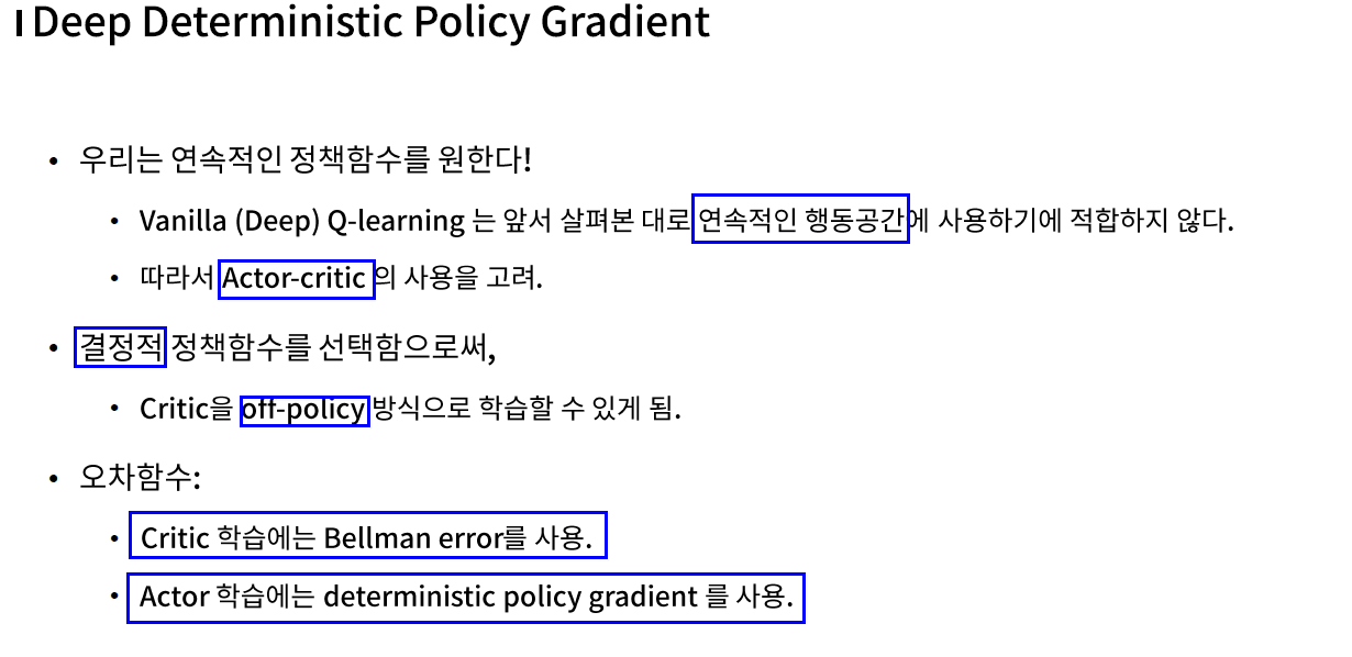
- “연속적인 (continuous)” action space를 다룰 수 있다
- Deterministic Policy 사용
- 1) Off-policy 가능
- 2) Efficient Sampling
- Ornstein-Uhlenbeck 과정 : “시간적 연관성”을 가지는 exploration technique
2. Deterministic Policy Gradient
“연속적인 (continuous)” action space를 Q-learning에서 다룰 수 있는 방법?
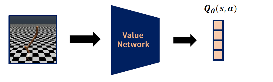
- 방법 1) continuous action space를 discretecize (이산화) 한다
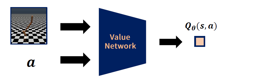
- 방법 2) action을 또 다른 input으로 간주
Q-learning
-
model free algorithm
-
\(Q(s, a) \leftarrow Q(s, a)+\eta\left(r+\gamma \max _{a^{\prime}} Q\left(s^{\prime}, a^{\prime}\right)-Q(s, a)\right)\).
방법 1) 행동 이산화
- \([-1,1]\) 의 action space를…
-
\([-1,-1+\Delta \mathrm{a},-1+2 \Delta \mathrm{a}, \ldots, 1]\)로 이산화
- 그런 뒤 일반적인 Q-Learning 적용하기
방법 2) Action을 또 다른 Input으로
-
Q-learning의 target에서 \(\max _{a^{\prime}} \boldsymbol{Q}_{\boldsymbol{\theta}}\left(s^{\prime}, a^{\prime}\right)\) 를 찾는건 매우 힘들다!
( \(\boldsymbol{Q}_{\boldsymbol{\theta}}\left(s^{\prime}, a^{\prime}\right)\)가 convex function이 아니므로! )
( \(A\)의 가지 수가 적었으면 그냥 해보면 됬지만….. continuous한 경우에는 사실상 hard )
1) 궁극적으로 구하고자 하는 것 : continuous policy \(\pi (a \mid s)\)
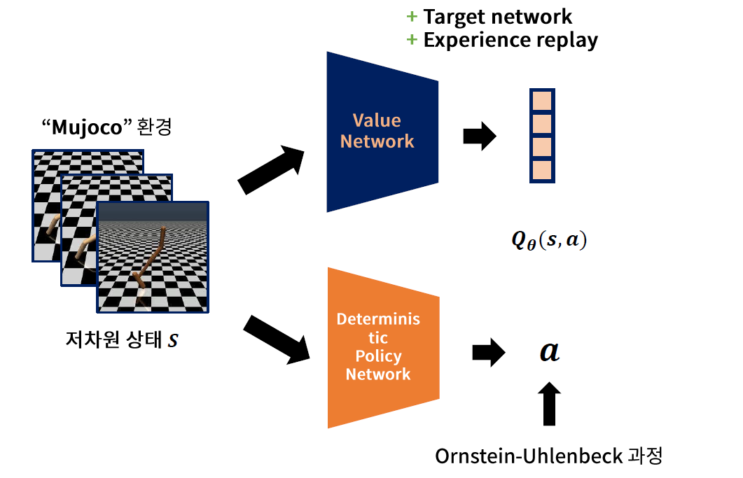
\(\rightarrow\) Actor-Critic을 사용해보자!
- Actor : “Deterministic” policy function
- Critic : Q-Network
Deterministic의 장점
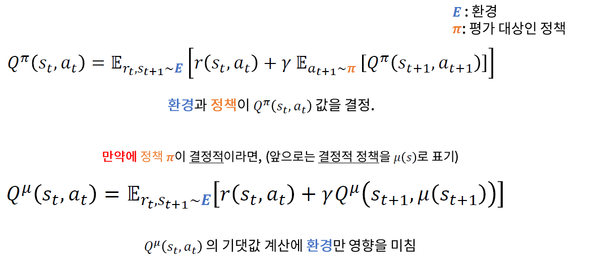
\(\rightarrow\) 기댓값 계산에 환경만이 영향을 미치므로, Off-policy 학습이 가능해진다!
요약 : (1) “연속적’‘이면서 (2) “결정적”“인 정책을 학습하자!
2) Policy Gradient 복습
\(p\left(s \rightarrow s^{\prime}, t, \pi\right)\).
- 현재 상태 \(s\)에서, 정책 \(\pi\) 하에서, \(t\) 시점 후에 \(s'\)에 도달할 확률
\(\rho^{\pi}\left(s^{\prime}\right) \stackrel{\text { def }}{=} \int_{s \in \mathcal{S}} \sum_{t=1}^{\infty} \gamma^{t-1} p_{1}(s) p\left(s \rightarrow s^{\prime}, t, \pi\right) d s\).
-
(감가된) 상태의 분포
-
\(s\)에서 \(s'\)에 도달할 확률 ( 시간 고려 )
( 즉, 너무 먼 미래라면, 가능성이 낮다는 사실을 반영 )
Loss Function
(1) Stochastic
\(\begin{aligned} J\left(\pi_{\theta}\right) &=\int_{s \in S} \rho^{\pi_{\theta}}(s) \int_{a \in \mathcal{A}} \pi_{\theta}(s, a) r(s, a) d a d s =\mathbb{E}_{s \sim \rho^{\pi} \theta, a \sim \pi_{\theta}}[r(s, a)] \end{aligned}\).
(2) Deterministic
\(\begin{aligned} J\left(\mu_{\theta}\right) &=\int_{s \in \mathcal{S}} \rho^{\mu_{\theta}}(s) r\left(s, \mu_{\theta}(s)\right) d s =\mathbb{E}_{s \sim \rho^{\pi} \theta}\left[r\left(s, \mu_{\theta}(s)\right)\right] \end{aligned}\).
\(\rightarrow\) \(J\left(\mu_{\theta}\right)\)에 대한 gradient는?
Gradient of Loss Function
\(\begin{aligned} \nabla_{\theta} J\left(\mu_{\theta}\right) &=\left.\int_{S \in \mathcal{S}} \rho^{\mu_{\theta}}(s) \nabla_{\theta} \mu_{\theta}(s) \nabla_{a} Q(s, a)\right|_{a=\mu_{\theta}(s)} d s \\ &=\mathbb{E}_{s \sim \rho} \pi_{\theta}\left[\left.\nabla_{\theta} \mu_{\theta}(s) \nabla_{a} Q(s, a)\right|_{a=\mu_{\theta}(s)}\right] \end{aligned}\).
위 식을 계산하기 위해서는..
- \(\nabla_{\theta} \mu_{\theta}(s)\)…..\(\theta\)에 대해 편미분을 계산하기 쉬운 “deterministic” 정책 함수 \(\mu_{\theta}(s)\)
- \(\nabla_{a} Q(s, a)\)……..\(a\)에 대해 편미분을 계산하기 쉬운 \(Q(s,a)\)
\(\rightarrow\) NN으로 모델링하자!
Summary
3. Ornstein-Uhlenbeck 과정을 통한 Exploration
(핵심) Determinstic policy를 통해 Off-policy 사용
Random Policy \(\rightarrow\) TOO LONG time
\(\therefore\) 시간적 연관성을 고려한 Ornstein-Uhlenbeck 과정을 사용한다!
직관적 이해 :
수식적 이해
- 시간적으로 서로 연관된 확률 변수 생성
- \(d x_{t}=-\theta x_{t} d t+\sigma d W_{t}\).
- \(\frac{d x_{t}}{d t}=-\theta x_{t}+\sigma \eta(t)\).
- \(\eta(t)\) : white noise
4. Summary