[ Recommender System ]
18. Variational Autoencoders for Collaborative Filtering
( 참고 : Fastcampus 추천시스템 강의 )
paper : Variational Autoencoders for Collaborative Filtering ( Liang et al., 2018 )
( https://arxiv.org/pdf/1802.05814.pdf )
선행 지식 : variational autoencoder, variational inference ( seunghan96.github.io 에서 참고! )
Abstract
VAE + CF
- generative model with Multinomial likelihood
- Variational Inference 사용
기존의 모델보다 우수한 성능!
1. Model
DLGM (Deep Latent Gaussian Model) 과 유사! 알고리즘은 매우 심플하다.
1) 각 user \(u\)에 대해, \(K\)-dim의 latent vector를 샘플링 :
- \[\mathbf{z}_{u} \sim \mathcal{N}\left(0, \mathbf{I}_{K}\right)\]
2) non-linear 함수 (\(f_{\theta}(\cdot)\) , 주로 NN으로 사용 )
- \(\pi\left(\mathbf{z}_{u}\right) \propto \exp \left\{f_{\theta}\left(\mathbf{z}_{u}\right)\right\}\).
- 이후 softmax를 통해 normalize ( 이후에 확률 parameter로 사용되기 때문에! )
3) 위의 output을 Multinomial의 parameter로써 사용
- \(\mathbf{x}_{u} \sim \operatorname{Mult}\left(N_{u}, \pi\left(\mathbf{z}_{u}\right)\right)\).
위의 모델은, 기존의 Gaussian과 Logistic보다 뛰어난 성능을 보인다.
- Gaussian ) \(\log p_{\theta}\left(\mathbf{x}_{u} \mid \mathbf{z}_{u}\right) \stackrel{c}{=}-\sum_{i} \frac{c_{u i}}{2}\left(x_{u i}-f_{u i}\right)^{2}\).
- Logistic ) \(\log p_{\theta}\left(\mathbf{x}_{u} \mid \mathbf{z}_{u}\right)=\sum_{i} x_{u i} \log \sigma\left(f_{u i}\right)+\left(1-x_{u i}\right) \log \left(1-\sigma\left(f_{u i}\right)\right)\).
2. Variational Inference
위 1에서 알아본 것은, \(z\)로 \(x'\)을 복원하는 generative model로 볼 수 있다.
이제 \(x\)로 \(z\)를 encoding하는 모델 ( inference model )에 대해서 알아볼 것이다.
이 모델에서는 variational distribution을 다음과 같이 Normal로 세팅한다.
\(q_{\phi}\left(\mathbf{z}_{u} \mid \mathbf{x}_{u}\right)=\mathcal{N}\left(\mu_{\phi}\left(\mathbf{x}_{u}\right), \operatorname{diag}\left\{\sigma_{\phi}^{2}\left(\mathbf{x}_{u}\right)\right\}\right)\).
VAE를 학습하기 위해, KL-divergence를 최소화해야한다. 이는 곧 ELBO를 최대화하는 것과 같다.
\(\begin{aligned} \log p\left(\mathbf{x}_{u} ; \theta\right) & \geq \mathbb{E}_{q_{\phi}\left(\mathbf{z}_{u} \mid \mathbf{x}_{u}\right)}\left[\log p_{\theta}\left(\mathbf{x}_{u} \mid \mathbf{z}_{u}\right)\right]-\operatorname{KL}\left(q_{\phi}\left(\mathbf{z}_{u} \mid \mathbf{x}_{u}\right) \| p\left(\mathbf{z}_{u}\right)\right) \\ & \equiv \mathcal{L}\left(\mathbf{x}_{u} ; \theta, \phi\right) \end{aligned}\).
-
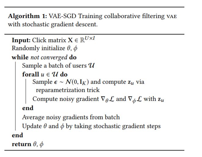
reparam trick 사용!
\(\mathbf{z}_{u}=\mu_{\phi}\left(\mathbf{x}_{u}\right)+\boldsymbol{\epsilon} \odot \sigma_{\phi}\left(\mathbf{x}_{u}\right)\) where \(\boldsymbol{\epsilon} \sim \mathcal{N}\left(0, \mathbf{I}_{K}\right)\)
알다시피, 위의 ELBO는 두개의 term으로 구성된다
- 1) reconstruction error term
- 2) KL-divergence term ( regularizer의 역할 )
위 ELBO식의 좀 더 general한 표현을 얻어보자. second term인 KL-divergence term앞에 parameter \(\beta\)를 줌으로써, regularize하고 싶은 강도를 조절할 수 있다.
\(\begin{aligned} \mathcal{L}_{\beta}\left(\mathbf{x}_{u} ; \theta, \phi\right) \equiv \mathbb{E}_{q_{\phi}\left(\mathbf{z}_{u} \mid \mathbf{x}_{u}\right)} \left[\log p_{\theta}\left(\mathbf{x}_{u} \mid \mathbf{z}_{u}\right)\right] -& \beta \cdot \operatorname{KL}\left(q_{\phi}\left(\mathbf{z}_{u} \mid \mathbf{x}_{u}\right) \| p\left(\mathbf{z}_{u}\right)\right) \end{aligned}\).
이 알고리즘은, 학습과정에 있어서 \(\beta\)를 0에서 1로 점차 올라가는 방법을 제안한다.
Algorithm