4.Model-based Collaborative Filtering

[ Recommender System ]

4. Model-based Collaborative Filtering

( 참고 : Fastcampus 추천시스템 강의 )

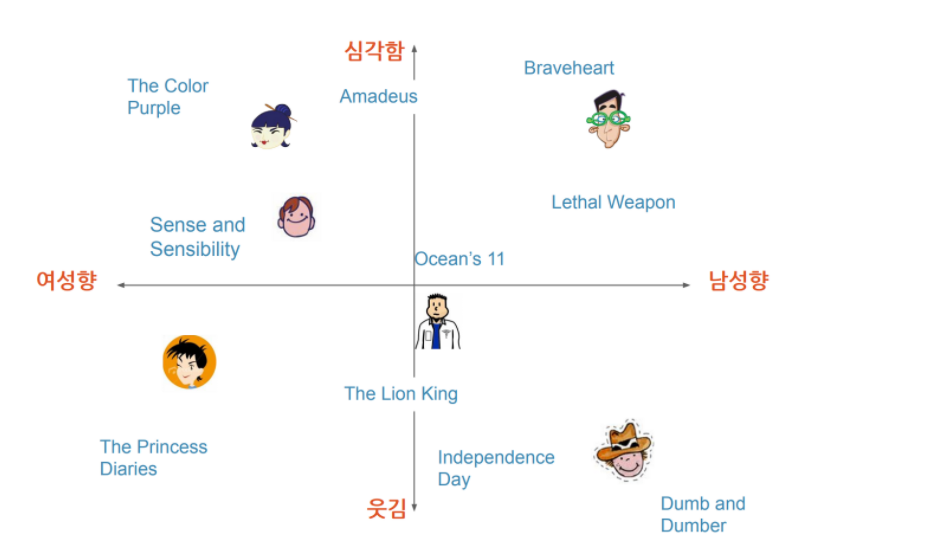
1. Latent Factor

latent factor : 잠재된 변수/factor

• User/Item의 vector representation으로 생각하면 된다

  ( into a lower dimension )

• 해당 vector space에서의 similarity/disimilarity를 파악!

2. SVD (Singular Value Decomposition)

( Linear Algebra에서 배운 개념을 복습해보자 )

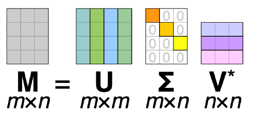
행렬 A는 다음과 같이 분해될 수 있다 : \(A = U\Sigma V^T\)

• \(U\)와 \(V\)는 orthogonal matrix
  • \(U\)의 shape : \(m \times m\)
  • \(V\)의 shape : \(n \times n\)
• \(\Sigma\)는 diagonal matrix
  • \(\Sigma\)의 shape : \(m \times n\)
  • 대각원소 : eigen-value의 제곱근 ( = A의 특이값 )

이를 추천시스템에 적용해보자면,

• \(U\)는 User의 latent factor
• \(V\)는 Item의 latent factor로 볼 수 있다

3. Matrix Factorization

앞서 언급한 latent factor model을 구현하는 방법으로, (추천시스템의 관점에서) Rating Matrix를 아래와 같이 분해하는 것을 의미한다

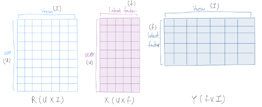
Notation 소개

• \(R\) : Rating Matrix ( shape : \(U \times I\) )

  ( where \(U\) = user의 수 & \(I\) : item의 수 )

• \(X\) : User의 latent factor matrix ( shape : \(U \times f\) )

• \(Y\) : Item의 latent factor matrix ( shape : \(f \times I\) )

  ( where \(f\) = 줄이고 싶은 dimension )

• predicted rating : \(\hat{r_{ui}} = x_u^T \times y_i\)

  ( 여기서 구한 predicted rating을 통해 matrix의 빈 칸을 채워나가는 문제로 볼 수 있다 )

정답인 \(R\) (rating matrix)와, 우리가 예측한 결과값인 \(R'\) (predicted matrix)간의 오차를 최소화하는 과정으로 모델을 학습한다.

Other SVD method

• SVD ++ , thin SVD, truncated SVD…

Optimization 방법으로는 대표적으로 아래와 같은 2가지 방법이 있다

• Stochastic Gradient Descent (SGD)
• Alternating Least Squares (ALS)

추가적인 정보를 사용하여 모델링할 수 있다

• Explicit feedback
• Implicit feedback

4. Objective Function of Matrix Factorization

Loss Function : \(\min \sum_{(u, i) \in T}\left(r_{u i}-x_{u}^{T} y_{i}\right)^{2}+\lambda\left(\left\|x_{u}\right\|^{2}+\left\|y_{i}\right\|^{2}\right)\)

• \(x_{u}, y_{i}:\) user와 item latent vector
• \(r_{u i}:\) user u가 item i에 부여한 REAL rating
• \(\widehat{r_{u i}}=x_{u}^{T} y_{i}:\) user u가 item i에 부여한(할) PREDICTED rating
• \(\lambda\left(\left\|x_{u}\right\|^{2}+\left\|y_{i}\right\|^{2}\right):\) overfitting 방지를 위한 일종의 penalty/regularization term

5. Optimization of Matrix Factorization

5-1. SGD (Stochastic Gradient Descent)

Error term을 줄여나가는 방식으로 \(x_u\) & \(y_i\)를 update!

​ ( update gradient of Loss function w.r.t \(x_u\) & \(y_i\) )

Error term :

​ \(e_{u i}=r_{u i}-x_{i}^{T} y_{u}\)

Updating Equation :

​ \(\begin{array}{l} x_{u} \leftarrow x_{u}+\gamma\left(e_{u i} \cdot y_{i}-\lambda \cdot x_{u}\right) \\ y_{i} \leftarrow y_{i}+\gamma\left(e_{u i} \cdot x_{u}-\lambda \cdot y_{i}\right) \end{array}\)

장점 : 구현이 쉽고, 계산이 빠르다

5-2. ALS (Alternating Least Squares)

대부분의 경우, \(x_u\)와 \(y_i\)를 둘 다 알수 없다. 따라서 풀어야 하는 문제는 non-convex하다.

이를 풀기 위해, \(x_u\)와 \(y_i\)를 교대로 하나는 고정하고, 하나는 update해가는 방식으로 문제를 풀어나간다.

이는 \(x_u\)와 \(y_i\)를 독립적으로 계산하기 때문에, 병렬적으로 처리할 수 있다.

6. Etc

위의 기본적인 Matrix Factorization에, 아래와 같은 variation들을 줄 수 있다.

ex) Adding Bias term

• \(\widehat{r_{u i}}=\mu+b_{i}+b_{u}+x_{u}^{T} y_{i}\).
  • \(\mu\) : 모든 Item의 평균
  • \(b_i\): 전체 Item 평균에 대한 Item \(i\)의 편차
  • \(b_u\): 전체 User평균에 대한 User \(u\)의 편차
• loss function : \(\min \sum_{(u, i) \in T}\left(r_{u i}-\mu-b_{i}-b_{u}-x_{u}^{T} y_{i}\right)^{2}+\lambda\left(\left\|x_{u}\right\|^{2}+\left\|y_{i}\right\|^{2}+b_{i}^{2}+b_{u}^{2}\right)\)

ex) Adding Additional Input

• additional input ?

  \(\sum_{i \in N(u)} y_{i}:\) User u의 Item i에 대한 implicit feedback

  ​ ( where \(N(u)\) : 전체 Item에 대한 User u의 implicit feedback )

  \(\sum_{a \in A(a)} x_{a}:\) User u의 personal or non-item related information

• \(\widehat{r_{u i}}=\mu+b_{i}+b_{u}+x_{u}^{T}\left[y_{i}+\mid N(u)\mid^{-0.5} \sum_{i \in N(u)} y_{i} \sum_{a \in A(u)} x_{a}\right]\).

ex) Temporal Dynamics

• 시간에 따른 변화 반영 가능! ( \(t\) : time )
• \[\widehat{r_{u i}(t)}=\mu+b_{i}(t)+b_{u}(t)+x_{i}^{T} y_{u}(t)\]

ex) Inputs with varying Confidence Levels

• 쉽게 말해, error term에 서로 다른 weight를 부여하는 것

  ( WHY? 선택을 많이 받은 item과, 별로 없는 item간에 차이를 부여하기 위해! )

• \[\min \sum_{(u, i) \in T} \underbrace{c_{u i}}\left(r_{u i}-\mu-b_{i}-b_{u}-x_{u}^{T} y_{i}\right)^{2}+\lambda\left(\left\|x_{u}\right\|^{2}+\left\|y_{i}\right\|^{2}+b_{i}^{2}+b_{u}^{2}\right)\]

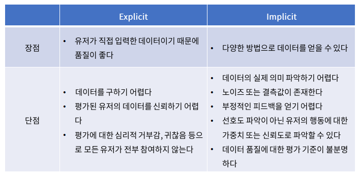
7. Explicit vs Implicit Feedback

model-based CF에서는, explicit info외에도 implicit info 또한 모델링에 사용할 수 있다.

각각의 info(feedback)의 장/단에 대해서 알아보자.