(paper) SSL05 - Temporal Ensembling

Temporal Ensembling for Semi-Supervised Learning (2017)

Contents

1. Abstract
2. Self-Ensembling during Training
   1. \(\Pi\)-model
   2. Temporal Ensembling

0. Abstract

simple and efficient method for training DNN

introduce self-ensembling

• form a consensus prediction of the unknown labels using the outputs of the network-in-training ….
  • on different epoch &
  • under different regularization and input augmentation conditions

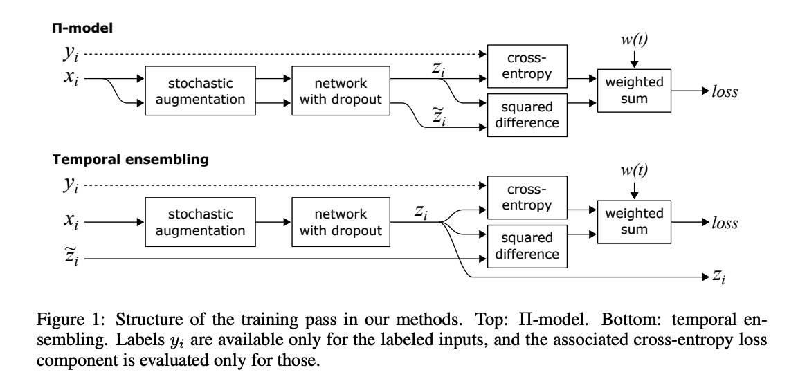
1. Self-Ensembling during Training

2 implementation during training

• (1) \(\Pi\)-model
  • encourages consistent network output between two realizations of the same input stimulus, under two different dropout conditions
• (2) temporal ensembling
  • simplifies and extends this by taking into account the network predictions over multiple previous training epochs

Notation

• \(N\) total inputs
  • \(M\) of them are labeled
• Training data : \(x_i\), where \(i \in\{1 \ldots N\}\).
• \(L\) : indicies of labeled inputs
  • \(\mid L\mid=M\).
  • for every \(i \in L\), we have a known correct label \(y_i \in\{1 \ldots C\}\)

(1) \(\Pi\)-model

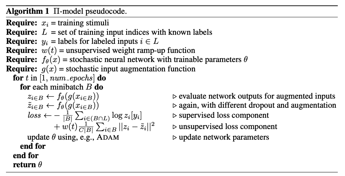
evaluate the network for each input \(x_i\) twice

• outputs : prediction vectors \(z_i\) and \(\tilde{z}_i\)

Loss function : consists of 2 components

• (1) standard CE ( for labeled input )
• (2) penalization ( for labeled & unlabeled input )
  • penalizes different predictions for the same input \(x_i\)
  • with MSE

(2) Temporal Ensembling

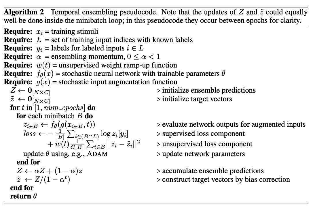
After every training epoch…

• the network outputs \(z_i\) are accumulated into ensemble outputs \(Z_i\)

  ( \(Z_i \leftarrow \alpha Z_i+(1-\alpha) z_i\) )

For generating the training targets \(\tilde{z}\)…

• correct for the startup bias in \(Z\) by dividing by factor \(\left(1-\alpha^t\right)\)