Neural Oblivious Decision Ensembles for DL on Tabular Data

Neural Oblivious Decision Ensembles for DL on Tabular Data

https://arxiv.org/pdf/1909.06312.pdf

Contents

1. Abstract

Abstract

Heterogeneous tabular data…

\(\rightarrow\) advantage of DNN over shallow algorithms is questionable!

NODE (Neural Oblivious Decision Ensembles)

• new deep learning achitectures with any tabular data
• ensemble of oblivious DT
  • (1) end-to-end GD training
  • (2) power of multi-layer hierarchical representation learning

1. Introduction

SOTA : shallow models ( ex. XGBoost )

\(\rightarrow\) DL methods do not consistently outperform SOTA models

NODE

• inspired by CatBoost
  • gradeint boosting on oblivious decision trees
• generalizes CatBoost
  • make splitting feature choice & decision tree routing differentiable
• resembles “deep” GBDT trained end-to-end
• via entmax transformation, perform soft splitting effectively

2. Related Works

(1) SOTA for tabular

GBDT, XGBoost, LightGBM

(2) Oblivious Decision Trees

Oblivious Decision Trees

• regular tree of depth \(d\)

• constrained to use the same splitting feature& threshold in all internal nodes of the same depth

  \(\rightarrow\) significantly weak learners & efficient

(3) Differentiable Trees

End-to-end optimization ( via softening decision functions )

(4) Entmax

maps a vector of real-valued scores to discrete prob distn

• capable to produce sparse probability distns

  ( majority of probabilities are exactly equal to 0 )

learn splitting decisions based on a small subset of features

(5) Multi-layer non-differentaible architectures

Multi-layer GBDT (Feng et al., 2018)

• limitaiton: does not require each alyer compoenent to be differentiable

3. NODE

consists of differentiable ODT

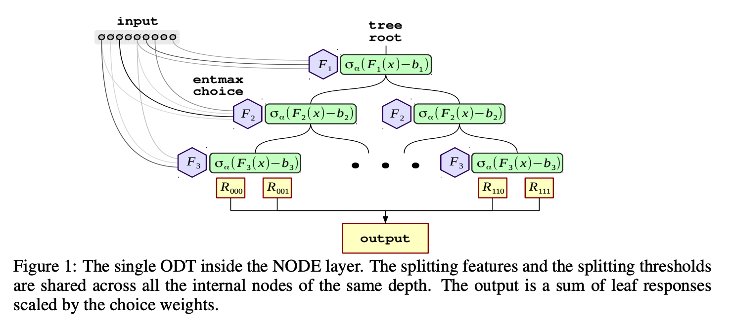
(1) Differentiable ODT

Notation

• \(M\): number of ODT

• \(d\) : depth of ODT

  ( = \(d\) splitting features = \(2^d\) possible responses )

• \(n\) : number of (numeric) features

• \(x \in \mathbb{R}^n\) : input vector

each ODT is determinbed by its ..

• splitting features \(f \in \mathbb{R}^d\)

• splitting thresholds \(b \in \mathbb{R}^d\)

• \(d\)-dimensional tensor of responses \(R \in \mathbb{R}^{\underbrace{2 \times 2 \times 2}_d}\).

Output of ODT:

• \(h(x)=R\left[\mathbb{1}\left(f_1(x)-b_1\right), \ldots, \mathbb{1}\left(f_d(x)-b_d\right)\right]\).
  • where \(\mathbb{1}(\cdot)\) denotes the Heaviside function.

To make trees differentiable ….

• replace \(\mathbb{1}\left(f_i(x)-b_i\right)\) by their continuous counterparts

• ex)

  • REINFORCE (Williams, 1992)
  • Gumbel-softmax (Jang et al., 2016)

  \(\rightarrow\) require long training time… use \(\alpha\)-entmax transformation (Peters et al., 2019)

Entmax transformation

• replaced by a weighted sum of features
  • weights : computed as entmax over the learnable feature selection matrix \(F \in \mathbb{R}^{d \times n}\) :
• \(\hat{f}_i(x)=\sum_{j=1}^n x_j \cdot \operatorname{entmax}_\alpha\left(F_{i j}\right)\).

Relax the Heaviside function \(\mathbb{1}\left(f_i(x)-b_i\right)\) as a two-class entmax

• \(\sigma_\alpha(x)=\operatorname{entmax}_\alpha([x, 0])\).
• use the scaled version: \(c_i(x)=\sigma_\alpha\left(\frac{f_i(x)-b_i}{\tau_i}\right)\)
  • where \(b_i\) and \(\tau_i\) are learnable parameters for thresholds and scales respectively.

Based on the \(c_i(x)\) values, we define a “choice” tensor \(C \in \mathbb{R}^ \underbrace{2 \times 2 \times 2}_d\)

\(C(x)=\left[\begin{array}{c} c_1(x) \\ 1-c_1(x) \end{array}\right] \otimes\left[\begin{array}{c} c_2(x) \\ 1-c_2(x) \end{array}\right] \otimes \cdots \otimes\left[\begin{array}{c} c_d(x) \\ 1-c_d(x) \end{array}\right]\).

[ Final prediction ]

\(\hat{h}(x)=\sum_{i_1, \ldots i_d \in\{0,1\}^d} R_{i_1, \ldots, i_d} \cdot C_{i_1, \ldots, i_d}(x)\).

• weight : \(R\)
• response : \(C\)

[ Output of the NODE layer ]

\(\left[\hat{h}_1(x), \ldots, \hat{h}_m(x)\right]\).

( = concatenation of the outputs of \(m\) individual trees )

Multi-dimensional tree outputs

( Above: output = 1-dim )

For cls task, output = \(C\) -dim

\(\rightarrow\) multidimensional tree outputs \(\hat{h}(x) \in \mathbb{R}^{\mid C \mid}\)

• where \(\mid C \mid\) is a number of classes.

(2) Going Deeper with NODE

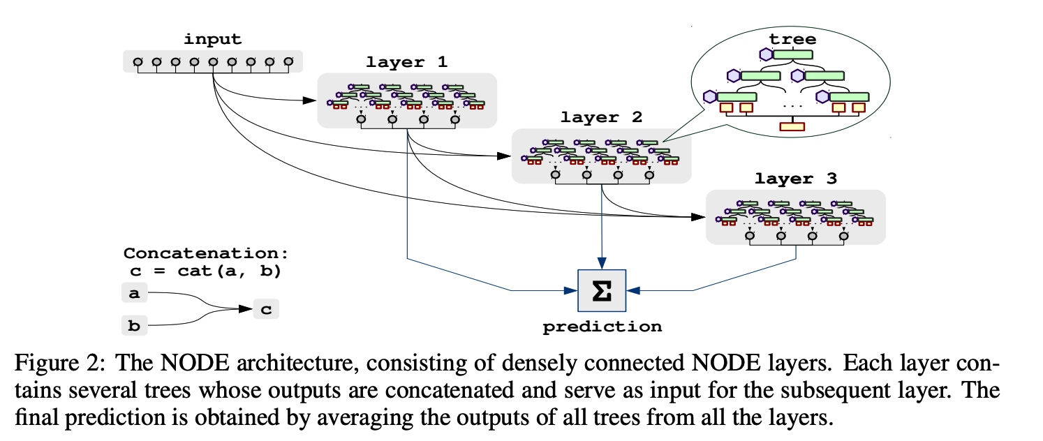
( Similar to DenseNet )

• sequence of \(k\) NODE layers
• concatenate all previous layers as its inputs

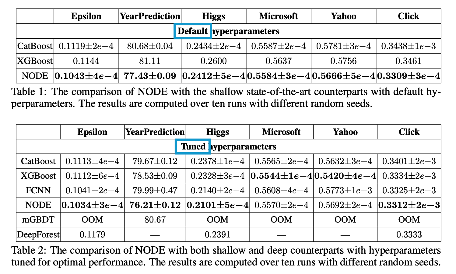
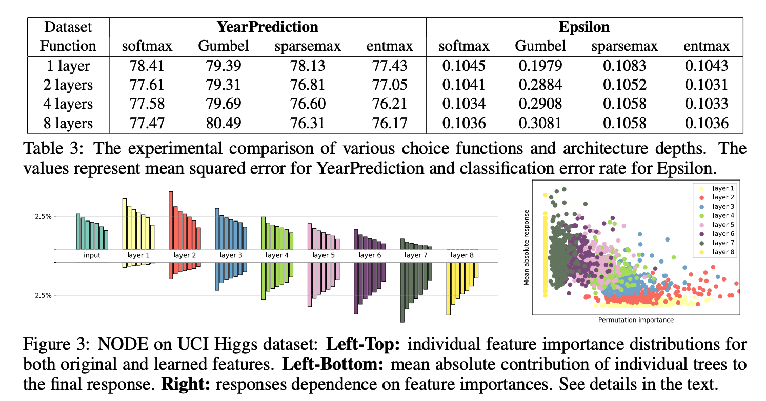
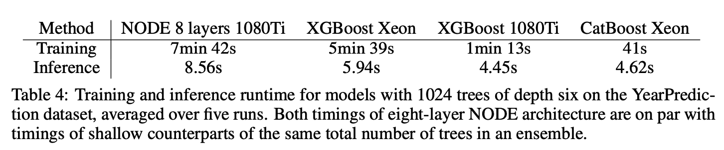
4. Experiments