SAINT; Improved Neural Networks for Tabular Data via Row Attention and Contrastive Pre-training

SAINT: Improved Neural Networks for Tabular Data via Row Attention and Contrastive Pre-training

https://arxiv.org/pdf/2106.01342.pdf

Contents

1. Introduction
2. Related Works
   1. Classical models
   2. Deep tabular models
   3. Axial attention
3. SAINT
   1. Architecture
   2. Intersampel attention
4. Pre-training & Finetuning
5. Experimental Evaluation

Abstract

SAINT ( Self-Attention and Intersample Attention Transformer )

• Hybrid deep learning approach to solving tabular data problems
• Details:
  • performs attention over both ROWS and COLUMNS
  • includes an enhanced embedding method
• Propose new contrastive self-supervised pre-training method

1. Introduction

Q) Why DL suffer in Tabular data?

1. often contain heterogeneous features

   • mixture of continuous, categorical, and ordinal values

     ( these values can be independent or correlated )

2. no inherent positional information in tabular data

   ( = order of columns is arbitrary … differs from NLP & CV )

   \(\rightarrow\) must handle features from multiple discrete and continuous distributions

   \(\rightarrow\) must discover correlations without relying on the positional information.

3. without performant deep learning models for tabular data, we lack the ability to exploit compositionality, end-to-end multi-task models, fusion with multiple modalities (e.g. image and text), and representation learning.

SAINT ( Self-Attention and Intersample Attention Transformer )

• specialized architecture for learning with tabular data

• leverages several mechanisms to overcome the difficulties of training on tabular data.

  • projects all features – categorical and continuous – into a combined dense vector space.

    • passed as tokens into a transformer encoder

  • Hybrid attention mechanism

    • (1) self-attention : attends to individual features within each data sample

    • (2) inter-sample attention : enhances the classification of a row (i.e., a data sample) by relating it to other rows in the table.

      ( = akin to a nearest-neighbor classification, where the distance metric is learned end-to-end rather than fixed )

• also leverage self-supervised contrastive pre-training

2. Related Works

(a) Classical Models

• pass

(b) Deep Tabular Models

TabNet [1]

• uses NN to mimic decision trees by placing importance on only a few features at each layer
• attention layers :
  • regular dot-product self-attention (X)
  • sparse layer that allows only certain features to pass through (O)

VIME [49]

• employs MLPs in a technique for pre-training based on denoising

TABERT [48]

• a more elaborate neural approach inspired by BERT
• trained on semi-structured test data to perform language-specific tasks

TabTransformer [18]

• learn contextual embeddings only on “categorical features”
• continuous features : concatenated to the embedded features
  • do not go through the self-attention block
  • correlations between categorical and continuous features is lost

SAINT

• project BOTH continuous features and categorical features

  & passing them to the transformer blocks

• propose a new type of attention

  • to explicitly allow data points to attend to each other to get better representations.

(c) Axial Attention

Axial Attention [17]

• first to propose ROW & COLUMN attention in the context of localized attention in 2D inputs (like images) in their Axial Transformer

• attention is computed only on the pixels that are on the same row and column

  ( rather than using all the pixels in the image )

MSA Transformer [33]**

• extends this work to protein sequences
• applies both column and row attention across similar rows (tied row attention)

TABBIE [20]

• adaptation of axial attention that applies self-attention to rows and columns separately,

  then averages the representations,

  and passes them as input to the next layer.

\(\rightarrow\) Different features from the same data point communicate with each other and with the same feature from a whole batch of data.

SAINT: propose intersample attention

• hierarchical in nature
• step 1) features of a given data point interact with each other
• step 2) data points interact with each other using entire rows/samples.

3. SAINT

Notation

• \(\mathcal{D}=\left\{\mathbf{x}_{\mathbf{i}}, y_i\right\}_{i=1}^m\) : tabular dataset with \(m\) points

• \(x_i\) : \(n\)-dimensional feature vector

• \(\mathbf{x}_{\mathbf{i}}=\left[ \text{[cls]} , f_i^{\{1\}}, f_i^{\{2\}}, . ., f_i^{\{n\}}\right]\) be a single data-point
• like BERT, append [CLS] token with a learned embedding
• single data-point with categorical or continuous features \(f_i^{\{j\}}\)
• \(\mathbf{E}\) : embedding layer that embeds each feature into a \(d\)-dim
• \(\mathbf{E}\) may use different embedding functions for different features
• Given \(\mathbf{x}_{\mathbf{i}} \in \mathbb{R}^{(n+1)}\), we get \(\mathbf{E}\left(\mathbf{x}_{\mathbf{i}}\right) \in \mathbb{R}^{(n+1) \times d}\).

Encoding the Data

NLP ) all tokens are embedded using the same procedure

Tabular) different features can come from distinct distributions

\(\rightarrow\) need a heterogeneous embedding approach

TabTransformer[18]

• uses attention to embed only categorical features

SAINT

• also projecting continuous features into a \(d\)-dim space before transformer
• use a separate single FC layer with a ReLU nonlinearity for each continuous feature
  • ( = projecting the 1-dim to \(d\)-dim )

(1) Architecture

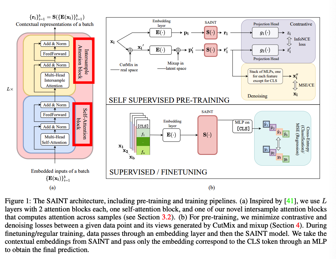
Composed of a stack of \(L\) identical stages

• 1 stage = 1 self-attention transformer block + 1 intersample attention transformer block

• (1) self-attention transformer block : identical as Transformer

  • multi-head self-attention layer (MSA) (with \(h\) heads) + 2 FC layer + GeLU

    ( each layer: skip connection + layer norm )

• (2) intersample attention transformer block :

  • same as (1), but self-attention layer is replaced by an intersample attention layer (MISA).

Notation:

• Single stage \((L=1)\) and a batch of \(b\) inputs
• MSA: multi-head self-attention
• MISA: multi-head intersample attention
• FF: feed-forward layers
• LN: layer norm

\(\mathbf{z}_{\mathbf{i}}^{(\mathbf{1})}=\operatorname{LN}\left(\operatorname{MSA}\left(\mathbf{E}\left(\mathbf{x}_{\mathbf{i}}\right)\right)\right)+\mathbf{E}\left(\mathbf{x}_{\mathbf{i}}\right)\).

\(\mathbf{z}_{\mathbf{i}}^{(\mathbf{2})}=\mathrm{LN}\left(\mathrm{FF}_1\left(\mathbf{z}_{\mathbf{i}}^{(\mathbf{1})}\right)\right)+\mathbf{z}_{\mathbf{i}}^{(\mathbf{1})}\).

\(\mathbf{z}_{\mathbf{i}}^{(\mathbf{3})}=\operatorname{LN}\left(\operatorname{MISA}\left(\left\{\mathbf{z}_{\mathbf{i}}^{(\mathbf{2})}\right\}_{i=1}^b\right)\right)+\mathbf{z}_{\mathbf{i}}^{(\mathbf{2})}\).

Final representation ( of data point \(\mathbf{x_i}\) )

• \(\mathbf{r}_{\mathbf{i}}=\mathrm{LN}\left(\mathrm{FF}_2\left(\mathbf{z}_{\mathbf{i}}^{(3)}\right)\right)+\mathbf{z}_{\mathbf{i}}^{(3)}\).
• used for downstrema tasks

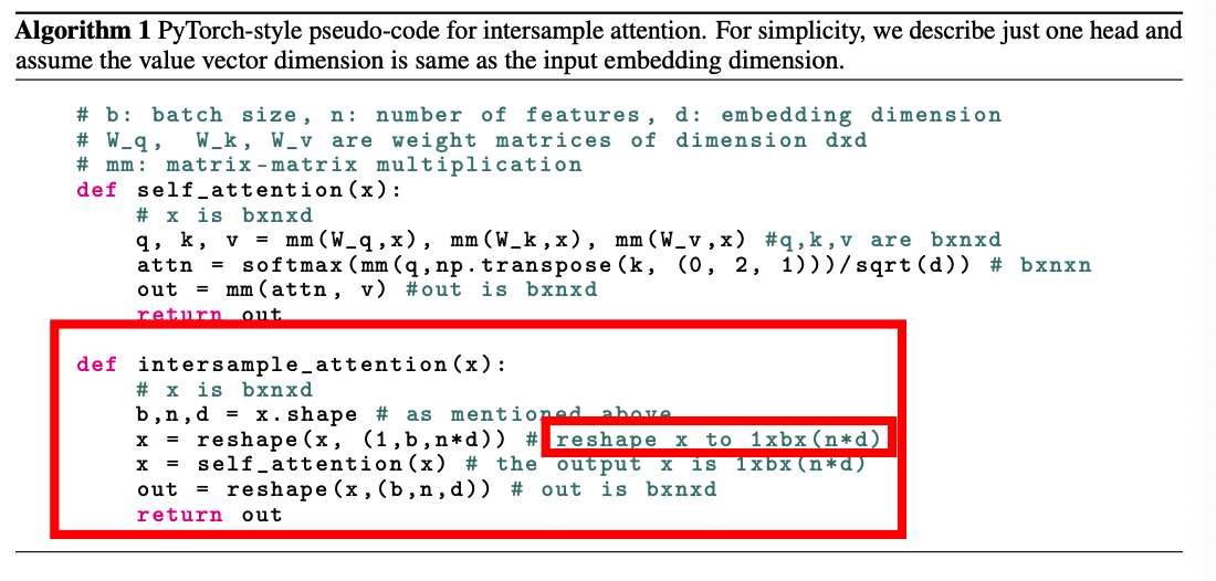
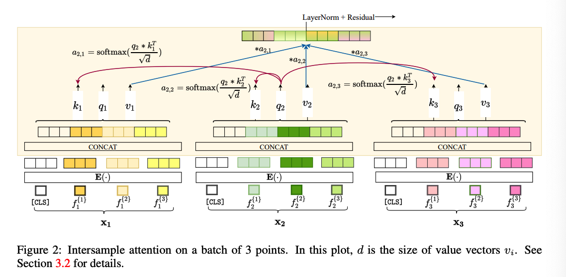
(2) Intersample Attention ( = ROW attention )

Attention is computed across different data points ( in a given batch )

Procedures

• (1) concatenate the embeddings of each feature for a single data point
• (2) compute attention over samples (rather than features).

Improve the representation of a given point by inspecting other points

Missing data?

• intersample attention enables SAINT to borrow the corresponding features from other similar data samples in the batch.

Experiments ) this ability boosts performance appreciably.

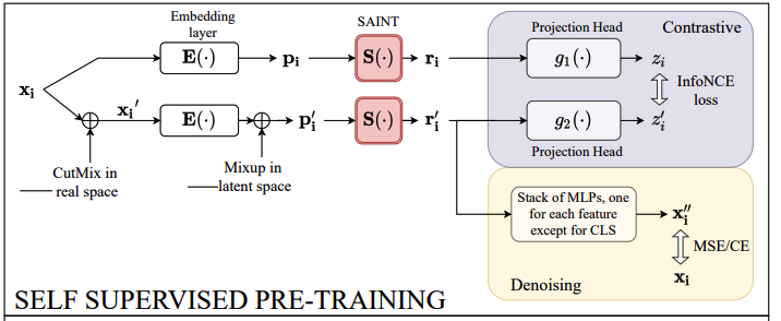
4. Pre-training & Finetuning

Present a contrastive pipeline for tabular data

Existing works ( on tabular data )

• denoising [43]
• variation of denosing: VIME [49]
• masking, and replaced token detection as used by TabTransformer [18]

\(\rightarrow\) still… superior results are achieved by contrastive learning

a) Generating augmentations

VIME [49]

• use mixup in the input space
• limited to continuous data

SAINT: use CutMix [50]

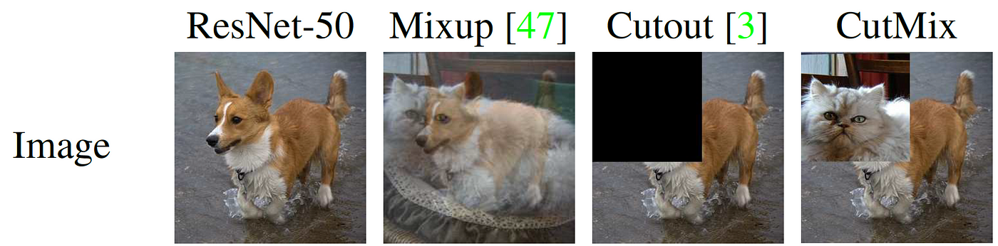
• https://sh-tsang.medium.com/paper-cutmix-regularization-strategy-to-train-strong-classifiers-with-localizable-features-5527e29c4890

2 augmentations:

• augment samples in the input space and we use mixup [51] in the embedding space
• challenging and effective self-supervision task

Notation:

• only \(l\) of \(m\) data points are labeled.
• embedding layer: \(\mathbf{E}\)
• SAINT network: \(\mathbf{S}\)
• 2 projection heads: \(g_1(\cdot)\) and \(g_2(\cdot)\).
• CutMix augmentation probability :\(p_{\text {cutmix }}\)
  • mixup parameter: \(\alpha\).

Two embeddings

• Original embedding : \(\mathbf{p}_{\mathbf{i}}=\mathbf{E}\left(\mathbf{x}_{\mathbf{i}}\right)\)
• Augmented embedding :
  • CutMix in raw data space : \(\mathbf{x}_{\mathbf{i}}^{\prime}=\mathbf{x}_{\mathbf{i}} \odot \mathbf{m}+\mathbf{x}_{\mathbf{a}} \odot(\mathbf{1}-\mathbf{m})\).
    • where \(\mathbf{x}_{\mathbf{a}}, \mathbf{x}_{\mathbf{b}}\) are random samples from the current batch
    • \(\mathbf{m}\) is the binary mask vector with probability \(p_{\text {cutmix }}\)
  • Mixup in the embdding space: \(\mathbf{p}_{\mathbf{i}}^{\prime}=\alpha * \mathbf{E}\left(\mathbf{x}_{\mathbf{i}}^{\prime}\right)+(1-\alpha) * \mathbf{E}\left(\mathbf{x}_{\mathbf{b}}^{\prime}\right)\).
    • \(\mathbf{x}_{\mathbf{b}}^{\prime}\) is the CutMix version of \(\mathbf{x}_{\mathbf{b}}\)

b) SAINT and projection heads

Pass both \(\mathbf{p}_{\mathbf{i}}\) and mixed \(\mathbf{p}_{\mathbf{i}}^{\prime}\) embeddings to SAINT

• 2 projection heads ( each head = 1 MLP + ReLU )

  • use of a projection head to reduce dimensionality before computing CL is common in CV

    & indeed also improves results on tabular data.

c) Loss functions

2 losses for the pre-training phase

• contrastive loss ( from InfoNCE loss )
• denoising task ( predict the original data sample from a noisy view )

\(\mathcal{L}_{\text {pre-training }}=-\sum_{i=1}^m \log \frac{\exp \left(z_i \cdot z_i^{\prime} / \tau\right)}{\sum_{k=1}^m \exp \left(z_i \cdot z_k^{\prime} / \tau\right)}+\lambda_{\mathrm{pt}} \sum_{i=1}^m \sum_{j=1}^n\left[\mathcal{L}_j\left(\mathbf{M L P}_j\left(\mathbf{r}_{\mathbf{i}}^{\prime}\right), \mathbf{x}_{\mathbf{i}}\right)\right]\).

• where \(\mathbf{r}_{\mathbf{i}}=\mathbf{S}\left(\mathbf{p}_{\mathbf{i}}\right), \mathbf{r}_{\mathbf{i}}^{\prime}=\mathbf{S}\left(\mathbf{p}_{\mathbf{i}}^{\prime}\right), z_i=g_1\left(\mathbf{r}_{\mathbf{i}}\right), z_i^{\prime}=g_2\left(\mathbf{r}_{\mathbf{i}}^{\prime}\right)\).
• \(\mathcal{L}_j\) = CE or MSE loss ( depending on the \(j^{\text {th }}\) feature )

d) Finetuning

Finetune the model on the target prediction task using the \(l\) labeled samples

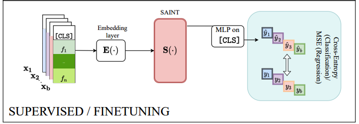
Given \(\mathbf{x}_{\mathbf{i}}\), learn the contextual embedding \(\mathbf{r}_{\mathbf{i}}\).

Final prediction step:

• pass the embedding corresponding only to the [CLS] token
• via a single MLP with a single hidden layer with ReLU

5. Experimental Evaluation

Summary

• 16 tabular datasets.

• Variants of SAINT
  • in both supervised and semi-supervised scenarios

• Analyze each component of SAINT

• Ablation studies

• Visualization ( to interpret the behavior of attention maps )

Datasets

14 binary classification tasks & 2 multiclass classification tasks

• size : 200 to 495,141
• features : 8 to 784
  • with both categorical and continuous features
• some datasets are missing data
• some are well-balanced while others have highly skewed class distributions.
• pre-processing step :
  • continuous : Z-normalized,
  • categorical : label-encoded

Model variants

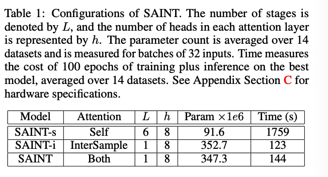
SAINT-i : only intersample attention

SAINT-s : is exactly the encoder from vanilla Transformer

Baselines

• Logistic regression

• Random forests

• XGBoost, LightGBM, and CatBoost

• MLP, VIME, TabNet, and TabTransformer

Pretraining tasks

• TabNet: MLM
• TabTransformer: Replaced Token Detection (RTD)
• MLP: use denoising [43] as suggested in VIME.

Metrics

majority of the tasks : binary classification

• primary measure : AUROC
  • captures how well the model separates the two classes in the dataset.

two multi-class datasets ( Volkert and MNIST)

• measure : accuracy

(1) Results

a) Supervised setting

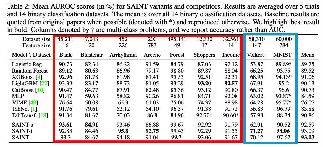
• 7 binary classification & 2 multiclass classification
• 5 trials with different seeds

b) Semi-supervised setting

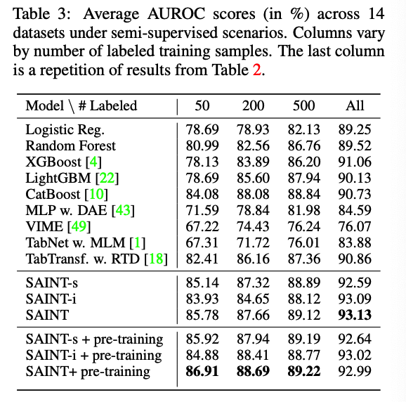
3 set of experiments

• 50, 200, 500 labeled data points

c) Effect of embedding continuous features

Perform a simple experiment with TabTransformer

• Modify TabTransformer by embedding continuous features into \(d\)-dimensions using a single layer ReLU MLP

Results ( average AUROC )

• original TabTransformer : 89.38
• original TabTransformer + embedding the continuous features : 91.72

\(\rightarrow\) embedding the continuous data is important

d) When to use intersample attention?

SAINT-i

• consistently outperforms other variants whenever the number of features is large

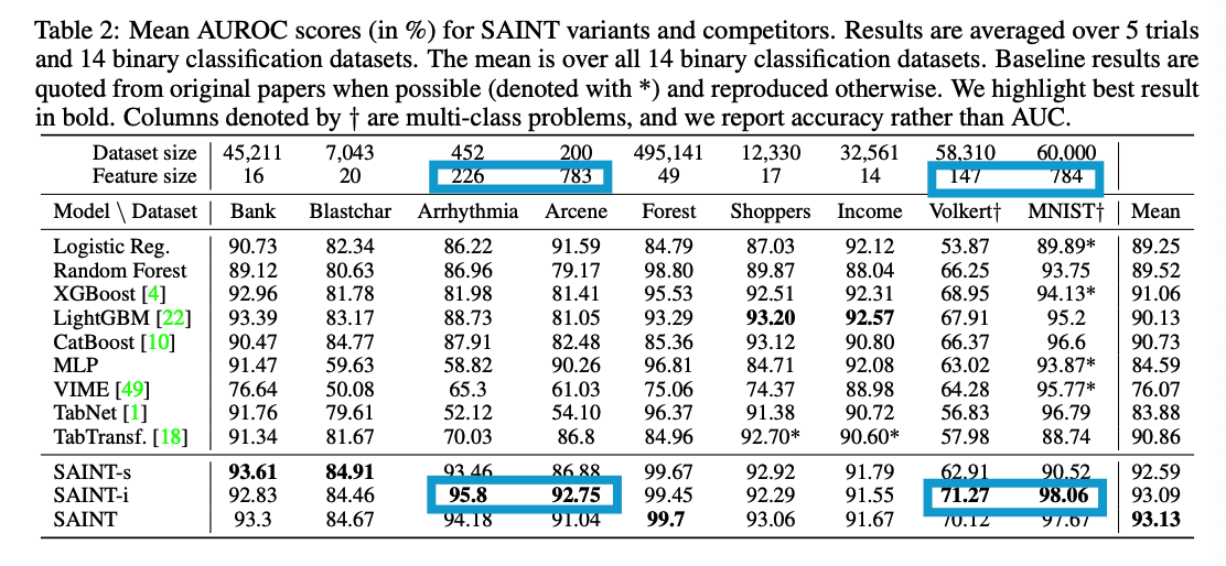
Whenever there are few training data points + many features (common in biological datasets)

\(\rightarrow\) SAINT-i outperforms SAINT-s significantly (see the “Arcene” and “Arrhythmia” results).

Pros & Cons

• pros) faster compared to SAINT-s

• cons) number of parameters is much higher than that of SAINT-s

e) How robust is SAINT to data corruptions?

To simulate corruption, we apply CutMix

• replacing 10% to 90% of the features with values of other randomly selected samples

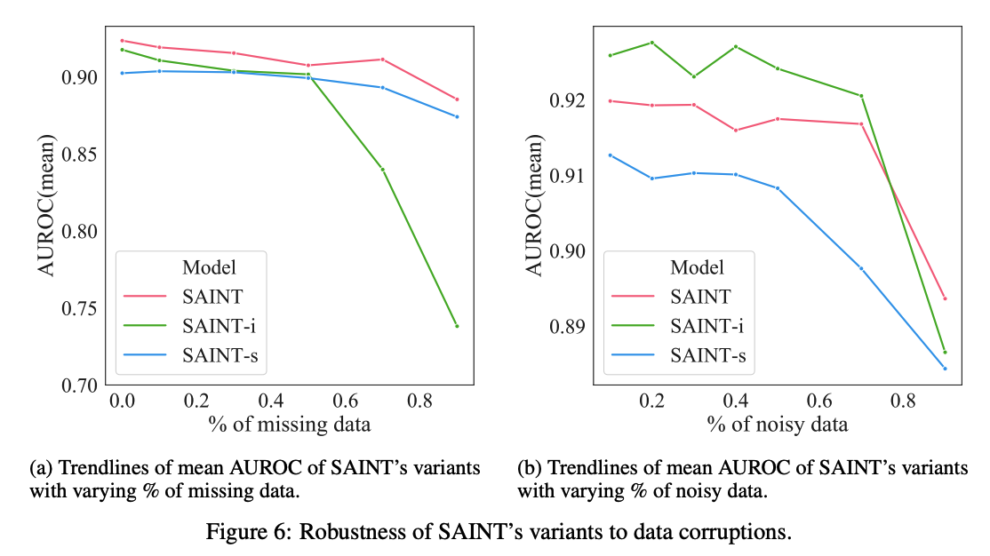
\(\rightarrow\) (RIGHT) noisy data: ROW attention improves the model’s robustness to noisy training data

\(\rightarrow\) (LEFT) missing data: opposite trend

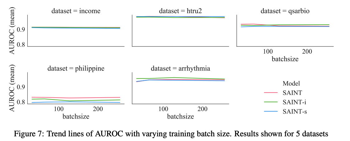
f) Effect of batch size