TransTab; Learnable Transferable Tabular Transformers across Tables

TransTab: Learnable Transferable Tabular Transformers across Tables (NeurIPS 2022)

https://arxiv.org/pdf/2205.09328.pdf

Contents

1. Introduction
2. Method
   1. Application scenarios of TransTab
   2. Input processor for columns and cells
   3. Gated Transformers
   4. SSL pretraining

Abstract

Questions

• How to learn ML models from multiple tables with partially overlapping columns?

• How to incrementally update ML models as more columns become available over time?

• Can we leverage model pretraining on multiple distinct tables?

• How to train an ML model which can predict on an unseen table?

Answer

• Propose to relax fixed table structures by introducing a Transferable Tabular Transformer (TransTab) for tables.

TransTab

• convert each sample to a generalizable embedding vector
  • apply stacked transformers for feature encoding.
• Insight )
  • (1) combining column description and table cells as the raw input to a gated transformer model.
  • (2) introduce supervised and self-supervised pretraining

1. Introduction

Existing works :

• require the same table structure in training and testing data

\(\rightarrow\) HOWEVER … there can be multiple tables sharing partially overlapped columns

Rethink the basic elements in tabular data modeling

Basic elements

• CV) pixel / patches
• NLP) words / tokens
• Tabular) it is natural to treat cells in each column as independent

Existing works

• Columns are mapped to unique indexes & models take the cell values for training and inference.
  • assumption) keep the same column structure in all the tables.

\(\rightarrow\) tables often have divergent protocols where the nomenclatures of columns and cells differ.

\(\rightarrow\) \(\therefore\) proposed work contextualizes the columns and cells

Example

• previous methods ) codebook {man : 0, woman : 1}
• proposed ) converts the tabular input into a sequence input (e.g., gender is man)

\(\rightarrow\) such featurizing protocol is generalizable across tables!

\(\rightarrow\) enable models to apply to different tables.

Transferable Transformers for Tabular analysis (TransTab)

a versatile tabular learning framework

• applies to multiple use cases

Key contributions

• systematic featurizing pipeline considering both column and cell semantics
  • shared as the fundamental protocol across tables.
• Vertical-Partition Contrastive Learning (VPCL)
  • enables pretraining on multiple tables & allows finetuning on target datasets

2. Method

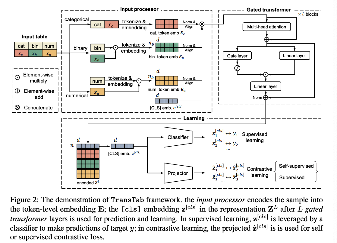
Key components:

1. Input processor
   • featurizes and embeds arbitrary tabular inputs to token-level embeddings
2. Stacked gated transformer layers
   • further encode the token-level embeddings
3. Learning module
   • classifier ( trained on labeled data )
   • projector ( for contrastive learning )

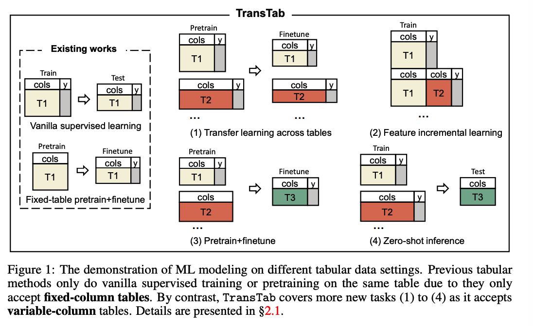
(1) Application scenarios of TransTab

S(1) Transfer learning.

• collect data tables from multiple cancer trials

  & testi the efficacy of the same drug on different patients

• designed independently with overlapping columns

• How do we learn ML models for one trial by leveraging tables from all trials?

S(2) Incremental learning

• Additional columns might be added over time.

S(3) Pretraining+Finetuning

• The trial outcome label (e.g., mortality) might not be always available
• Can we benefit pretraining on those tables without labels?

S(4) Zero-shot inference.

• model the drug efficacy based on our trial records
• next step) conduct inference with the model to find patients that can benefit from the drug
• NOTE THAT patient tables do not share the same columns as trial tables

(2) Input processor for columns and cells

Input processor

• (1) accept variable-column tables
• (2) to retain knowledge across tabular datasets

Key Idea: convert tabular data into a sequence of semantically encoded tokens

How to create sequence?

• via the column description (e.g., column name)
  • ex) cell value 60 in column weight indicates \(60 \mathrm{~kg}\) in weight instead of 60 years old

Treats ANY tabular data as compotion of 3 elements

• (1) Text (for categorical \& textual cells and column names)
• (2) Continuous values (for numerical cells)
• (3) Boolean values (for binary cells).

a) Categorical/Textual feature

Contains a sequence of text tokens

\(\rightarrow\) concatenate the (1) column name with the (2) feature value \(x_c\) ( = becomes sentence )

\(\rightarrow\) then tokenized and matched to the token embedding matrix

Feature embedding \(\mathbf{E}_c \in \mathbb{R}^{n_c \times d}\)

• where \(d\) is the embedding dimension & \(n_c\) is the number of tokens.

b) Binary feature

Usually an assertive description & and its value \(x_b \in\{0,1\}\)

If \(x_b=1\)

• bin is tokenized and encoded to the embeddings \(\mathbf{E}_b \in \mathbb{R}^{n_b \times d}\)

If \(x_b=0\)

• will not be processed to the subsequent steps

\(\rightarrow\) significantly reduces the computational and memory cost .

c) Numerical feature

DO NOT concatenate column names and values for numerical feature. WHY?

\(\because\) the tokenization-embedding paradigm was notoriously known to be bad at discriminating numbers

( instead, process them separately (

num is encoded as \(\mathbf{E}_{u, c o l} \in\) \(\mathbb{R}^{n_u \times d}\).

Then, multiply the numerical features with the column embedding

Numerical embedding : \(\mathbf{E}_u=x_u \times \mathbf{E}_{u, c o l}\),

d) Merge

• \(\mathbf{E}_c, \mathbf{E}_u, \mathbf{E}_b\) all pass the layer normalization & same linear layer to be aligned to the same space
• then concatenated with [cls] embedding

\(\rightarrow\) \(\mathbf{E}=\tilde{\mathbf{E}}_c \otimes \tilde{\mathbf{E}}_u \otimes \tilde{\mathbf{E}}_b \otimes \mathbf{e}^{[c l s]}\).

(3) Gated Transformers

2 main components

• (1) multi-head self-attention layer
• (2) gated feedforward layers

Input representation \(\mathbf{Z}^l\) ( at the \(l\)-th layer )

\(\begin{array}{r} \mathbf{Z}_{\text {att }}^l=\text { MultiHeadAttn }\left(\mathbf{Z}^l\right)=\left[\operatorname{head}_1, \operatorname{head}_2, \ldots, \operatorname{head}_h\right] \mathbf{W}^O, \\ \operatorname{head}_i=\text { Attention }\left(\mathbf{Z}^l \mathbf{W}_i^Q, \mathbf{Z}^l \mathbf{W}_i^K, \mathbf{Z}^l \mathbf{W}_i^V\right), \end{array}\).

• where \(\mathbf{Z}^0=\mathbf{E}\) at the first layer
• \(\mathbf{W}^O \in \mathbb{R}^{d \times d} ;\left\{\mathbf{W}_i^Q, \mathbf{W}_i^K, \mathbf{W}_i^V\right\}\) are weight matrices (in \(\mathbb{R}^{d \times \frac{d}{h}}\) ) of query, key, value of the \(i\)-th head

Multi-head attention output \(\mathbf{Z}_{\text {att }}^l\)

• \(\mathbf{g}^l=\) \(\sigma\left(\mathbf{Z}_{\mathrm{att}}^l \mathbf{w}^G\right)\) : further transformed by a token-wise gating layer
  • \(\sigma(\cdot)\) : sigmoid function
  • \(\mathbf{g}^l \in[0,1]^n\) : the magnitude of each token embeddi
• \(\mathbf{Z}^{l+1}=\operatorname{Linear}\left(\left(\mathbf{g}^l \odot \mathbf{Z}_{\mathrm{att}}^l\right) \oplus \operatorname{Linear}\left(\mathbf{Z}_{\mathrm{att}}^l\right)\right)\).

Final \([\mathrm{cls}]\) embedding \(\mathbf{z}^{[c l s]}\) at the \(L\)-th layer is used by the classifier for prediction.

(4) SSL pretraining

Input processor accepts variable-column tables

\(\rightarrow\) enables tabular pretraining on heterogeneous tables

a) Self-supervised VPCL

Most SSL tabular methods

• work on the whole fixed set of columns
• high computational costs and are prone to overfitting

VPCL

• take tabular vertical partitions to build positive and negative samples for CL
• sample \(\mathbf{x}_i=\left\{\mathbf{v}_i^1, \ldots, \mathbf{v}_i^K\right\}\) with \(K\) partitions \(\mathbf{v}_i^k\).
  • Neighbouring partitions can have overlapping regions

Self-VPCL

• takes partitions from the same sample as the positive and others as the negative

• \(\ell(\mathbf{X})=-\sum_{i=1}^B \sum_{k=1}^K \sum_{k^{\prime} \neq k}^K \log \frac{\exp \psi\left(\mathbf{v}_i^k, \mathbf{v}_i^{k^{\prime}}\right)}{\sum_{j=1}^B \sum_{k^{\dagger}=1}^K \exp \psi\left(\mathbf{v}_i^k, \mathbf{v}_j^{k^{\dagger}}\right)}\).

  • \(B\) : the batch size
  • \(\psi(\cdot, \cdot)\) : cosine similarity function
  • \(\psi\) : linear projection ( applies to \(\hat{\mathbf{z}}^{[c l s]}\) , which is the linear projection of partition v’s embedding \(\mathbf{z}^{[c l s]}\). )

Effect

• significantly expand the positive and negative sampling
• extremely friendly to column-oriented databases
  • which support the fast querying a subset of columns from giant data warehouses.
• For the sake of computational efficiency, when \(K>2\), we randomly sample two partitions.

b) Supevised VPCL

build positive pairs considering views from the same class except for only from the same sample

( just like SupCON )

\(\ell(\mathbf{X}, \mathbf{y})=-\sum_{i=1}^B \sum_{j=1}^B \sum_{k=1}^K \sum_{k^{\prime}=1}^K \mathbf{1}\left\{y_j=y_i\right\} \log \frac{\exp \psi\left(\mathbf{v}_i^k, \mathbf{v}_j^{k^{\prime}}\right)}{\sum_{j^{\dagger}=1}^B \sum_{k^{\dagger}=1}^K \mathbf{1}\left\{y_{j^{\dagger}} \neq y_i\right\} \exp \psi\left(\mathbf{v}_i^k, \mathbf{v}_{j^{\dagger}}^{k^{\dagger}}\right)}\).

• \(\mathbf{y}=\left\{y_i\right\}_i^B\) are labels