Robust MTS Forecasting; Adversarial Attacks and Defense Mechanism

Abstract
Introduction
Related Work
1. Deep Forecasting Models
2. Adversarial Attack
Adversarial Attack Strategies
1. Framework on Sparse & Indirect Adversarial Attack
2. Deterministic Attack
3. Probabilistic Attack
Defense Mechanism against Adversarial Attacks
1. Randomized Smoothing Defense
2. Mini-max Defense

0. Abstract

Adversarial attack on MTS probabilistic forecasting & Defense mechanisms

This paper

[Attack] discover a new attack pattern
- by making strategic, sparse (imperceptible) modifications to the past observations
[Defense] Two defense strategies.
- (1) extend a previously developed randomized smoothing technique in CLS to FCST
- (2) develop an adversarial training algorithm
  - learns to create adversarial examples & optimize the forecasting model to improve its robustness

1. Introduction

Robustness for time-series models

Robustness = how sensitive the model output is when authentic data is (potentially) perturbed
In practice : corrupted by measurement noises,

Statistical forecasting models

less sensitive to such noises
more stable against outliers

$\rightarrow$ However, have not considered the possibility of adversarial noises which are strategically created

Not only in CLS, but also in FCST

ex) to mislead the forecasting of a particular stock, the adversaries might attempt to alter some features external to the stock’s financial valuation

Proposal

investigate such adversarial threats on more practical forecasting models
- whose predictions are based on more precise features, e.g. valuations of other stock indices.
- rather than releasing adverse information to alter the sentiment about the target stock on social media,
  
  the adversaries can instead invest hence change the valuation adversely

Adversarial perturbations & robustness should be defined more properly in TS setting.

few recent studies in this direction based on randomized smoothing (Yoon et al., 2022)

$\rightarrow$ restricted to univariate forecasting

( = make adverse alterations directly to the target TS )
MTS forecasting setup : remains unclear
- whether the attack to a target TS can be made instead via perturbing the other correlated TS
- whether it is defensible against such adversarial threats

3 questions:

(1) Indirect Attack.
- Can we mislead the prediction of some target TS via perturbations on the other TS?
(2) Sparse Attack.
- Can such perturbations be sparse and non-deterministic to be less perceptible?
(3) Robust Defense.
- Can we defend against those indirect and imperceptible attacks?

Technical contributions

a) Indirect attack

provide general framework of adversarial attack in MTS
devise a deterministic attack to the state-of-the-art probabilistic MTS forecasting model
- via adversely perturbing a subset of other TS
- via formulating the perturbation as solution of an optimization task with packing constraints.

b) Sparse attack

develop a non-deterministic attack that adversely perturbs a stochastic subset of TS related to the target TS
- makes the attack less perceptible.
- via a stochastic and continuous relaxation of the above packing constraint

c) Robust defense

propose 2 defense mechanisms.
(1) Randomized smoothing to the new MTS forecasting setup with robust certificate.
(2) Defense mechanism via solving a mini-max optimization task
- which minimizes the maximum expected damage caused by the probabilistic attack that continually updates the generation of its adverse perturbations in response to the model updates.

(1) Deep Forecasting Models

To model the uncertainty, various probabilistic models have been proposed

distributional outputs
distribution-free quantile-based outputs

(2) Adversarial Attack

DNN : vulnerable to adversarial attacks

even imperceptible adversarial noise can lead to completely different prediction.

CV : many adversarial attack schemes have been proposed

TS : much less literature

most existing studies on adversarial robustness of MTS models are restricted to regression and classification settings.
Yoon et al. (2022) studied both adversarial attacks to probabilistic forecasting models,
- but restricted to univariate settings

3. Adversarial Attack Strategies

Section

[3-1] Generic framework of sparse and indirect adversarial attack under a multivariate setting
[3-2] Deterministic attack
[3-3] Stochastic attack

Notation

Past MTS : $\mathbf{x}=\left\{\mathbf{x}_t\right\}_{t=1}^T \in \mathbb{R}^{d \times T}$
- $\mathbf{x}_t \in \mathbb{R}^d$.
- $x_{i, t}=\left[\mathbf{x}_t\right]_i$.
Future MTS : $\mathbf{z}=\left\{\mathbf{x}_{T+t}\right\}_{t=1}^\tau \in \mathbb{R}^{d \times \tau}$
Probabilistic forecaster : $p_\theta$
- takes history $\mathbf{x}$ to predict $\mathbf{z}$, i.e., $\mathbf{z} \sim p_\theta(\cdot \mid \mathbf{x})$.
We denote the set $[d]=\{1, \ldots, d\}$ and $i$-th time series as $\boldsymbol{\delta}^i=\left(\left[\boldsymbol{\delta}_t\right]_i\right)_{t=1}^T$.

(1) Framework on Sparse & Indirect Adversarial Attack

Given an adversarial prediction target $\mathbf{t}_{\mathrm{adv}}$ & historical input $\mathbf{x}$ to the forecaster $p_\theta(\mathbf{z} \mid \mathbf{x})$,

$\rightarrow$ design perturbation matrix $\boldsymbol{\delta}$

perturbed input $\mathbf{x}+\boldsymbol{\delta}$ disturbs a statistic $\chi(\mathbf{z})$ as close as possible to $\mathbf{t}_{\mathrm{adv}}$.

( = Goal : find $\boldsymbol{\delta}$ such that the distance between $\mathbb{E}_{\mathbf{z} \mid \mathbf{x}+\delta}[\chi(\mathbf{z})]$ and $\mathbf{t}_{\mathrm{adv}}$ is minimized )

Example )

$\chi(\mathbf{z})=\mathbf{z}$.
$\mathbf{t}_{\mathrm{adv}}=100 \mathbf{z}$.

$\rightarrow$ adversary’s target is to design an attack that can increase the prediction by 100 times.

Example )

suppose the adversaries want to mislead the forecasting of TS in a subset $\mathcal{I} \subset[d]$, denoted as $\mathbf{z}^{\mathcal{I}}$.
$\chi$ : bstatistic function of interest that concerns only time series in $\mathcal{I}$, i.e. $\chi(\mathbf{z})=\chi\left(\mathbf{z}^{\mathcal{I}}\right)$.
Sparse and indirect constraints

( = To make the attack less perceptible )
- (1) Perturbation $\delta$ cannot be direct to target TS in $\mathcal{I}$ and can be indirectly applied to a small subset of $\mathcal{I}^c=[d] \backslash \mathcal{I}$.
  - ( = restrict $\boldsymbol{\delta}^{\mathcal{I}}=\mathbf{0}$ and $s(\boldsymbol{\delta})=\mid\left\{i \in \mathcal{I}^c\right.$ : $\left.\delta^i \neq \mathbf{0}\right\} \mid \leq \kappa$ with sparsity level $\kappa \leq d$. )
- (2) Cap the energy of the attack
  - to avoid outlier detection
  - value of the perturbation at any coordinates is no more than a pre-defined threshold $\eta$.

$\rightarrow$ To sum up, the sparse and indirect attack $\delta$ can be found via solving

$\begin{array}{cc} \underset{\boldsymbol{\delta} \in \mathbb{R}^{T \times d}}{\operatorname{minimize}} & \{F(\boldsymbol{\delta}) \triangleq \mid \mid \mathbb{E}_{p_\theta(\mathbf{z} \mid \mathbf{x}+\boldsymbol{\delta})}[\chi(\mathbf{z})]-\mathbf{t}_{\mathrm{adv}} \mid \mid _2^2\} \\ \text { subject to } & \mid \mid \boldsymbol{\delta} \mid \mid _{\max } \leq \eta, s(\boldsymbol{\delta}) \leq \kappa, \boldsymbol{\delta}^{\mathcal{I}}=\mathbf{0}, \end{array}$.

small values of $\kappa$ and $\eta$ imply a less perceptible attack.
solving this is intractable due to the discrete cardinality constraint on $s(\boldsymbol{\delta})$.
develop two approximations
- (1) deterministic attack strategies.
- (2) non-deterministic attack strategies.

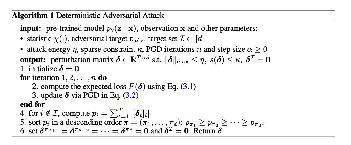
(2) Deterministic Attack

Approximated solution

Get an intermediate solution $\hat{\boldsymbol{\delta}}$

through projected gradient descent (PGD) until it converges,
$\hat{\boldsymbol{\delta}} \leftarrow \prod_{\mathcal{B}_{\infty}(0, \eta)}\left(\hat{\boldsymbol{\delta}}-\alpha \nabla_{\boldsymbol{\delta}} F(\hat{\boldsymbol{\delta}})\right),$.
- $\alpha \geq 0$ : a step size
- $\prod_{\mathcal{B}_{\infty}(0, \eta)}$ : the projection onto the $\ell_{\infty}$-norm ball with radius $\eta$,

With this intermediate non-sparse $\hat{\boldsymbol{\delta}}$,

retrieve for final sparse perturbation $\delta$ via solving

$\underset{\boldsymbol{\delta} \in \mathbb{R}^{T \times d}}{\operatorname{minimize}} \mid \mid \boldsymbol{\delta}-\hat{\boldsymbol{\delta}} \mid \mid _{\mathrm{F}} \quad \text { subject to } \quad s(\boldsymbol{\delta}) \leq \kappa, \boldsymbol{\delta}^{\mathcal{I}}=\mathbf{0} .$.
- can be solved analytically

Procedures

Compute the absolute perturbation added to each row $$i, p_i=\sum_{t=1}^T\left

\left[\hat{\boldsymbol{\delta}}_t\right]_i\right

$for$i \in[d] \backslash \mathcal{I}$$

Sort them in descending order $\pi: p_{\pi_1} \geq \cdots \geq p_{\pi_d}$.
Construct the solution as $\boldsymbol{\delta}$ with $\boldsymbol{\delta}^{\pi_i}=\hat{\boldsymbol{\delta}}^{\pi_i}$ if $i \leq \kappa$ else $\mathbf{0}$.

Remark.

$\nabla_\delta F(\boldsymbol{\delta})$ : doesn’t have a closed-form solution
Adopt the re-parameterized sampling approach

(3) Probabilistic Attack

Probabilistic sparse attack,

makes adverse alterations to a non-deterministic set of coordinates (i.e., time series and time steps).
appears to make the attack stronger and harder to detect.

View the sparse attack vector as a random vector drawn from a distribution with differentiable parameterization.

$\rightarrow$ Q) How to configure such a distribution whose support is guaranteed to be within the space of sparse vectors?

Propose “Sparse layer”

Distributional output
Dirac density combination.

a) Sparse Layer

Distributional output $q(\boldsymbol{\delta} \mid \mathbf{x} ; \beta, \gamma)$ of $\boldsymbol{\delta}$ having independent rows,
- such that its sample (probabilistic attack) $\boldsymbol{\delta} \sim q(\boldsymbol{\delta} \mid \mathbf{x} ; \beta, \gamma)=\prod_i q_i\left(\boldsymbol{\delta}^i \mid \mathbf{x} ; \beta, \gamma\right)$ satisfies sparse condition $\mathbb{E}[s(\boldsymbol{\delta})] \leq \kappa$ and $\boldsymbol{\delta}^{\mathcal{I}}=\mathbf{0}$.
parameterized by $\beta$ and $\gamma$
- $q_i\left(\boldsymbol{\delta}^i \mid \mathbf{x} ; \beta, \gamma\right) \triangleq r_i(\gamma) \cdot q_i^{\prime}\left(\boldsymbol{\delta}^i \mid \mathbf{x} ; \beta\right)+\left(1-r_i(\gamma)\right) \cdot D\left(\boldsymbol{\delta}^i\right)$.
  - $r_i(\gamma) \triangleq \kappa \gamma_i^{\frac{1}{2}} \cdot\left(\sum_{i=1}^d \gamma_i\right)^{-\frac{1}{2}} / \sqrt{d}$.
  - $D\left(\boldsymbol{\delta}^i\right)=\mathbb{I}\left(\boldsymbol{\delta}^i=\mathbf{0}\right)$.
  - $q_i^{\prime}\left(\boldsymbol{\delta}^i \mid \mathbf{x} ; \beta\right)$ : $\mathbb{N}\left(\mu(\mathbf{x} ; \beta), \sigma^2(\mathbf{x} ; \beta)\right)$
- combination weight $r_i(\gamma)$
  - probability mass of the event $\boldsymbol{\delta}^i=\mathbf{0}$,
  - means the choice of $\left\{r_i(\gamma)\right\}_{i=1}^d$ controls the row sparsity of the random matrix $\boldsymbol{\delta}$,
    - can be calibrated to enforce that $\mathbb{E}[s(\boldsymbol{\delta})] \leq \kappa$.

Implementation

$q_i^{\prime}(\cdot \mid \mathbf{x} ; \beta)$ : a distribution over dense vectors, e.g. $\mathbb{N}\left(\mu(\beta), \sigma^2(\beta) \mathbf{I}\right)$
$u_i \sim \mathbb{N}(0,1)$ for $i \in[d]$.
step 1) Construct a binary mask $m_i=\mathbb{I}\left(u_i \leq \Phi^{-1}\left(r_i(\gamma)\right)\right), i \in[d]$,
step 2) For each $i \in[d]$, we draw $\delta^{i^{\prime}}$ from $q_i^{\prime}(\cdot \mid \mathbf{x} ; \beta)$ and obtain $\delta^i$ by $\boldsymbol{\delta}^i=\boldsymbol{\delta}^{i^{\prime}} \cdot m_i$
step 3) set $\boldsymbol{\delta}^{\mathcal{I}}=\mathbf{0}$.

Optimizing Sparse Layer.

The differentiable parameterization can be optimized for maximum attack impact via minimizing the expected distance between the attacked statistic and adversarial target
$\min _{\beta, \gamma} H(\beta, \gamma) \triangleq \mathbb{E}_{\boldsymbol{\delta} \sim q(. \mid \mathbf{x} ; \beta, \gamma)} \mid \mid \mathbb{E}_{\mathbf{z} \sim p_\theta(\mathbf{z} \mid \mathbf{x}+\boldsymbol{\delta})}[\chi(\mathbf{z})]-\mathbf{t}_{\mathrm{adv}} \mid \mid _2^2 .$.

This attack is probabilistic in two ways.

(1) Magnitude
- magnitude of the perturbation $\delta$ is a random variable from distribution $q(\cdot \mid \mathbf{x})$.
(2) Components
- non-zero components of the mask depend on the random Gaussian samples

4. Defense Mechanisms against Adversarial Attacks

To enhance model robustness

via Randomized Smoothing
via Mini-max defense using sparse layer

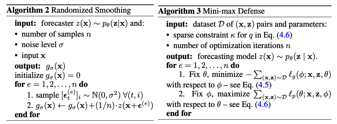
(1) Randomized Smoothing Defense

Randomized smoothing (RS)

post-training defense technique.
apply RS to our multivariate forecasters $z(\mathbf{x}) \sim p_\theta(\mathbf{z} \mid \mathbf{x})$
- maps $\mathbf{x}$ to a random vector $z(\mathbf{x})$

$\mathbb{P}_z(z(\mathbf{x}) \preceq \mathbf{r})$ : the CDF of such random outcome vector

$\preceq$ : the element-wise inequality

$g_\sigma(\mathbf{x})=\mathbb{E}_{\boldsymbol{\epsilon}}[z(\mathbf{x}+\boldsymbol{\epsilon})]$ : RS version of $z(\mathbf{x})$

random vector whose $\mathrm{CDF}$ is defined as $\mathbb{P}_{g_\sigma}\left(g_\sigma(\mathbf{x}) \preceq \mathbf{r}\right) \triangleq \mathbb{E}_{\boldsymbol{\epsilon} \mathbb{N}\left(\mathbf{0}, \sigma^2 \mathbf{I}\right)}\left[\mathbb{P}_z(z(\mathbf{x}+\boldsymbol{\epsilon}) \preceq \mathbf{r})\right]$
- noise level $\sigma>0$ and $\epsilon \sim \mathbb{N}\left(0, \sigma^2 \mathbf{I}\right)$
Computing the output of the smoothed forecaster $g_\sigma(\mathbf{x})$ is intractable
- since the integration of $z(\mathbf{x}+\boldsymbol{\epsilon})$ with $\mathbb{N}\left(0, \sigma^2 \mathbf{I}\right)$ cannot be done analytically.
- approximate using MC sampling

(2) Mini-max Defense

With a sparse layer $q(\cdot \mid \mathbf{x} ; \phi)$ having parameters $\phi=(\beta, \gamma)$

Train the forecaster by minimizing the worst-case loss caused by $q(\cdot \mid \mathbf{x} ; \phi)$ :

$\min _\phi \max _\theta \sum_{(\mathbf{x}, \mathbf{z}) \sim \mathcal{D}}\left[\ell_p(\theta ; \mathbf{x}, \mathbf{z}, \phi)-\ell_g(\phi ; \mathbf{x}, \mathbf{z}, \theta)\right]$.

Notation

$\ell_g(\phi ; \mathbf{x}, \mathbf{z}, \theta)$ : function of $\phi$ conditioned on $(\mathbf{x}, \mathbf{z}, \theta)$
$\ell_p(\theta ; \mathbf{x}, \mathbf{z}, \phi)$ : function of $\theta$ conditioned on $(\mathbf{x}, \mathbf{z}, \phi)$

$\begin{aligned} \ell_g(\phi ; \mathbf{x}, \mathbf{z}, \theta) & \triangleq \mathbb{E}_{q(\boldsymbol{\delta} \mid \mathbf{x} ; \phi)}\left[\mathbb{E}_{p_\theta\left(\mathbf{z}^{\prime} \mid \mathbf{x}+\boldsymbol{\delta}\right)} \mid \mid \mathbf{z}^{\prime}-\mathbf{z} \mid \mid ^2\right] \\ \ell_p(\theta ; \mathbf{x}, \mathbf{z}, \phi) & \triangleq \mathbb{E}_{q(\boldsymbol{\delta} \mid \mathbf{x} ; \phi)}\left[\log p_\theta(\mathbf{z} \mid \mathbf{x}+\boldsymbol{\delta})\right] \end{aligned}$.

mini-max defense

= finding a stable state where the model parameter is conditioned to perform best in the worst situation

= achieved by alternating between

(1) minimizing $-\ell_g$ with respect to $(\beta, \gamma)$

similar ideas have been previously exploited in GAN

Twitter Facebook LinkedIn

(paper 79) Robust MTS Forecasting; Adversarial Attacks and Defense Mechanism

Seunghan Lee

Robust MTS Forecasting; Adversarial Attacks and Defense Mechanism

Contents

0. Abstract

1. Introduction

Technical contributions

a) Indirect attack

b) Sparse attack

c) Robust defense

(1) Deep Forecasting Models

(2) Adversarial Attack

3. Adversarial Attack Strategies

Notation

(1) Framework on Sparse & Indirect Adversarial Attack

(2) Deterministic Attack

(3) Probabilistic Attack

a) Sparse Layer

4. Defense Mechanisms against Adversarial Attacks

(1) Randomized Smoothing Defense

(2) Mini-max Defense

You May Also Enjoy

(paper 79) Robust MTS Forecasting; Adversarial Attacks and Defense Mechanism

Seunghan Lee

Robust MTS Forecasting; Adversarial Attacks and Defense Mechanism

Contents

0. Abstract

1. Introduction

Technical contributions

a) Indirect attack

b) Sparse attack

c) Robust defense

2. Related Work

(1) Deep Forecasting Models

(2) Adversarial Attack

3. Adversarial Attack Strategies

Notation

(1) Framework on Sparse & Indirect Adversarial Attack

(2) Deterministic Attack

(3) Probabilistic Attack

a) Sparse Layer

4. Defense Mechanisms against Adversarial Attacks

(1) Randomized Smoothing Defense

(2) Mini-max Defense

You May Also Enjoy