(paper 96) Reversible Instance Normalization For Accurate Time Series Forecasting Against Distribution Shift

Reversible Instance Normalization For Accurate Time-Series Forecasting Against Distribution Shift (ICLR 2022)

https://openreview.net/pdf?id=cGDAkQo1C0p

Contents

1. Abstract
2. Introduction
3. Related Work
   1. TS Forecasting
   2. Distribution Shift
4. Proposed Method
   1. RevIN
   2. Effect of RevIN on Distn Shift
5. Experiments
   1. Experimental Setup
   2. Results and Analyses

Abstract

TS data suffer from a distribution shift

propose Reversible instance normalization (RevIN)

• simple yet effective normalization

• generally applicable normalization-and-denormalization method

  • with learnable affine transformation

1. Introduction

Distribution shift problem

• yield discrepancies between the distributions of the training and test data
• ex) TSF task
  • (input & output) training and test data are usually divided from the original data based on a specific point in time ( + hardly overlap )
  • (input & input) can have different underlying distributions as well

Remove non-stationary information from the input sequences ??

\(\rightarrow\) (PROBLEM) prevent the model from capturing the original data distn

• removes non-stationary information that can be important

\(\rightarrow\) (SOLUTION) explicitly return the information removed by input normalization back to the model

RevIN

propose to reverse the normalization applied to the input data in the output layer ( = denormalize )

• using the normalization statistics

Contributions

1. RevIN: simple yet effective normalization-and-denormalization method

   ( generally applicable with negligible cost. )

2. SOTA on 7 large-scale real-world datasets

3. Quantitative & Qualitative visualizations

2. Related Work

(1) TS Forecasting

• pass

(2) Distribution Shift

TSF models : suffer from non-stationary TS

• data distribution changes over time

Domain adaptation (DA) & Domain generalization (DG)

• common ways to alleviate the distribution shif
• DA vs. DG
  • DA : reduce the distribution gap between source and target
  • DG : only relies on the source domain
    • hopes to generalize on the target domain
• common objective : bridges the gap between source and target

Defining a domain is not straightforward in non-stationary TS

• since the data distribution shifts over time

Adaptive RNNs (Du et al., 2021)

( https://arxiv.org/pdf/2108.04443.pdf ( CIKM 2021 ) )

• handle the distribution shift problems of non-stationary TS

• step 1) characterizes the distribution information by splitting the training data into periods.

• step 2) matches the distributions of the discovered periods to generalize the model

• problem : COSTLY

  ( \(\leftrightarrow\) RevIN is simple yet effective and model-agnostic )

3. Proposed Method

Reversible instance normalization

• to alleviate the distribution shift problem in TS
  • discrepancy between the training and test data distn

Section Intro

• [ Section 3.1 ] proposed method
• [ Section 3.2 ] how it mitigates the distribution discrepancy in TS

(1) RevIN

Multivariate time-series forecasting task (MTSF task)

Input & Output

• input : \(\mathcal{X}=\left\{x^{(i)}\right\}_{i=1}^N\)
• output : \(\mathcal{Y}=\left\{y^{(i)}\right\}_{i=1}^N\)

Notation

• \(N\) : number of TS
• \(K\) : number of variables (channels)
• \(T_x\) : input length
• \(T_y\) : output length

Task: given \(x^{(i)} \in \mathbb{R}^{K \times T_x}\), predict \(y^{(i)} \in \mathbb{R}^{K \times T_y}\).

RevIN

• symmetrically structured normalization-and-denormalization layers

[ Process ]

step 1) normalize \(x^{(i)}\)

• instance-specific mean and standard deviation

  ( = instance normalization )

• \(\mathbb{E}_t\left[x_{k t}^{(i)}\right]=\frac{1}{T_x} \sum_{j=1}^{T_x} x_{k j}^{(i)}\).
• \(\operatorname{Var}\left[x_{k t}^{(i)}\right]=\frac{1}{T_x} \sum_{j=1}^{T_x}\left(x_{k j}^{(i)}-\mathbb{E}_t\left[x_{k t}^{(i)}\right]\right)^2\).

\(\rightarrow\) \(\hat{x}_{k t}^{(i)}=\gamma_k\left(\frac{x_{k t}^{(i)}-\mathbb{E}_t\left[x_{k t}^{(i)}\right]}{\sqrt{\operatorname{Var}\left[x_{k t}^{(i)}\right]+\epsilon}}\right)+\beta_k\).

• where \(\gamma, \beta \in \mathbb{R}^K\) are learnable affine parameter vectors

step 2) forward

• receives the transformed data \(\hat{x}^{(i)}\)
• forecasts their future values

step 3) de-normalize ( = reverse )

• explicitly return the non-stationary properties
• by reversing the normalization step at a symmetric position
• \(\hat{y}_{k t}^{(i)}=\sqrt{\operatorname{Var}\left[x_{k t}^{(i)}\right]+\epsilon} \cdot\left(\frac{\tilde{y}_{k t}^{(i)}-\beta_k}{\gamma_k}\right)+\mathbb{E}_t\left[x_{k t}^{(i)}\right]\).

Summary

1. effectively alleviate distribution discrepancy in TS

2. generally-applicable trainable normalization layer

3. most effective when applied to virtually symmetric layers of encoder-decoder structure

• boundary between the encoder and the decoder is often unclear

  \(\rightarrow\) apply RevIN to the input and output layers of a model

(2) Effect of RevIN on Distn Shift

RevIN can alleviate the distribution discrepancy, by

• (1) removing non-stationary information in the input layer
• (2) restoring it in the output layer

• analyze the distns of the training and test data at each step
• RevIN significantly reduces their discrepancy

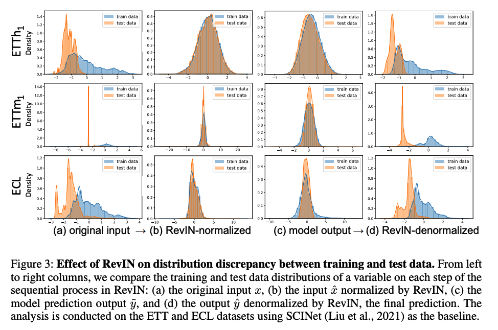
Summary of Figure 3

• Original input (Fig. 3(a))

  • train & test hardly overlap (especially ETTm1)

• Normalization step (Fig. 3(b))

  • transforms each data distribution into mean-centered distributions

    = supports that the original multimodal distributions (Fig. 3(a)) are caused by discrepancies in distributions between different sequences in the data

  • makes train & test data distributions overlapped.

• Prediction output (Fig. 3(c))

  • retain aligned training and test data distributions

• Denormalization step (Fig. 3(d))

  • returned back to the original distribution

  • w/o denormalization ??

    \(\rightarrow\) the model needs to reconstruct the values that follow the original distributions using only the normalized input ( NO non-stationary info )

Hypothesize that the distribution discrepancy will be reduced in the intermediate layers of the model as well ( Section 4.2.3 )

4. Experiments

(1) Experimental Setup

a) Datasets

• ETTh1, ETTh2, ETTm1, ECL(Electricity)
• Air quality ( from the UCI repository )
• Nasdaq ( from M4 competition )

b) Experimental details.

Prediction lengths

• ETTh1, ETTh2, ECL ( hourly-basis datasets )
  • 1d, 2d, 7d, 14d, 30d, and 40d
• ETTm1 : ( minute-bases datasets )
  • six hours (6h), 12h, 3d, 7d and 14d
• metric : MSE & MAE
  • compute the MSE and MAE on z-score

c) Baselines

3 SOTA TSF models ( = non-AR models )

• Informer (Zhou et al., 2021)
• N-BEATS (Oreshkin et al., 2020)
• SCINet (Liu et al., 2021)

Reproduction details ( Appendix A.12. )

• compare RevIN and the baselines under the same hyperparameter settings, including the input and prediction lengths.

(2) Results and Analyses

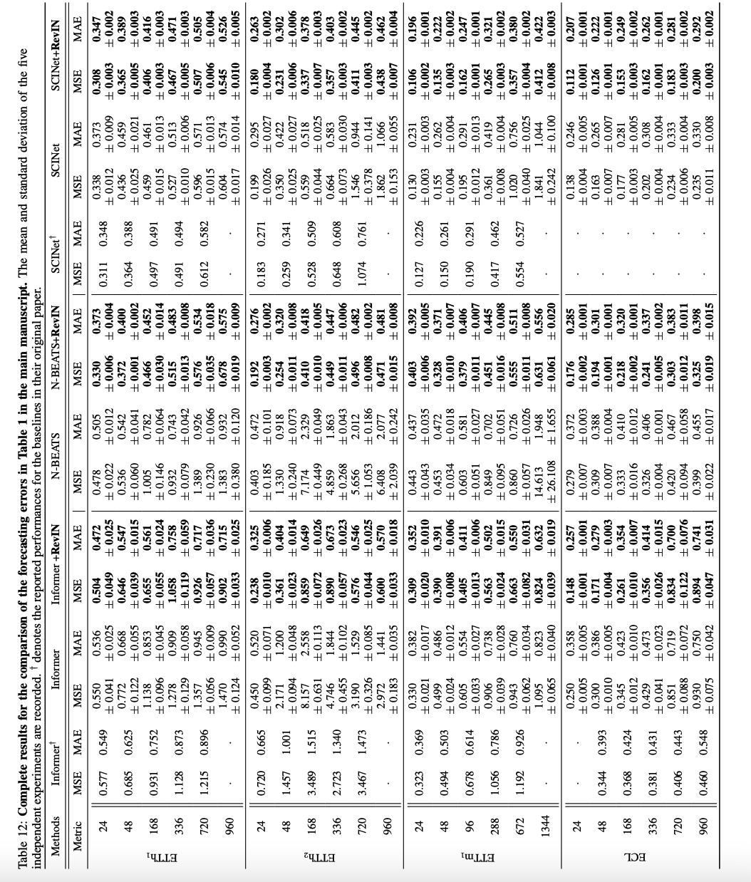
a) Effectiveness of RevIN on TSF models

• input length ( hyperparameter search )
  • ETTh, Weather, ELC : [24, 48, 96, 168, 336, 720]
  • ETTm : [24, 48, 96, 192, 288, 672]
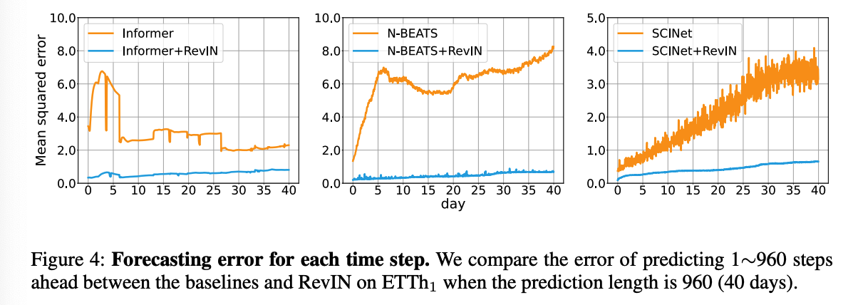
• effectiveness of RevIN is more evident for the long sequence prediction,
  • makes the baseline model more robust to prediction length

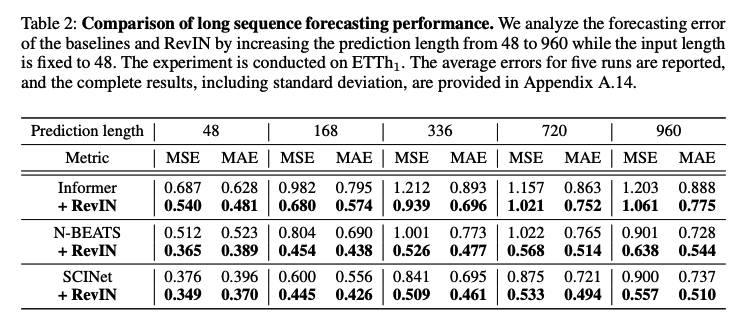
• input length : 48
• prediction length : [48,168,336,720,960]

How RevIN perform well in long sequence prediction ?

b) Comparision with existing normalization methods

Baseline methods

• min-max
• z-score
• layer norm
• batch norm
• instance norm
• DAIN ( deep adaptive input normalization )

Apply it on N-BEATS

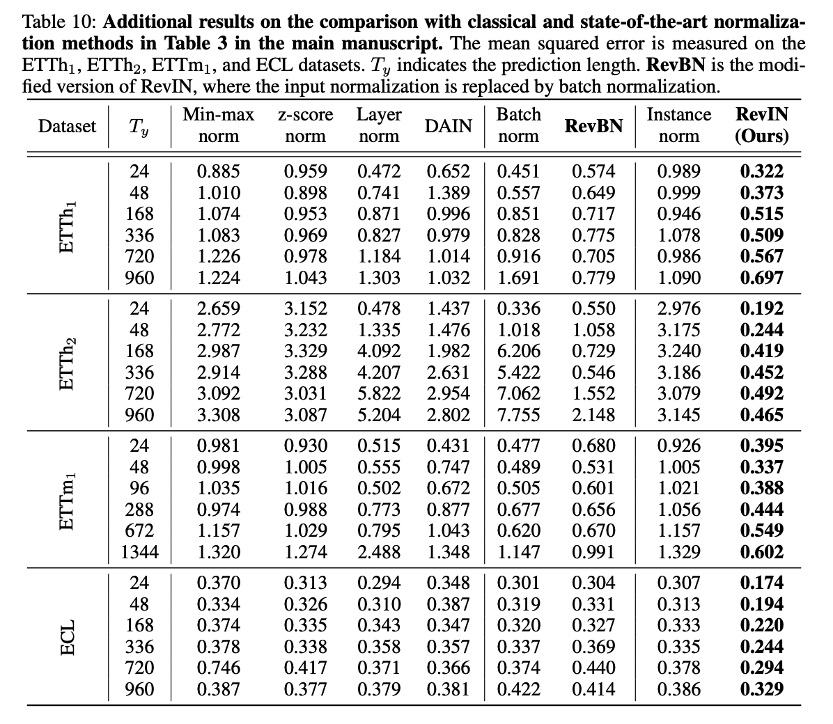
Batch Normalization (BN)

• applies identical normalization to all the input sequences

  ( = global statistics obtained from the entire training data )

  \(\rightarrow\) can not reduce the discrepancy between the train & test

Lightweight ( \(K\): num of variables )

• DAIN : \(3K^2\)
• RevIN : \(2K\)
• DishTS : \(2K\) + \(2KL\)
  • \(L\) : length of time series

c) Analysis of Distn shift in the Intermediate layers

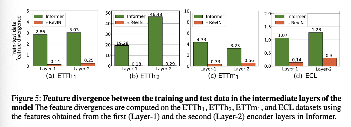
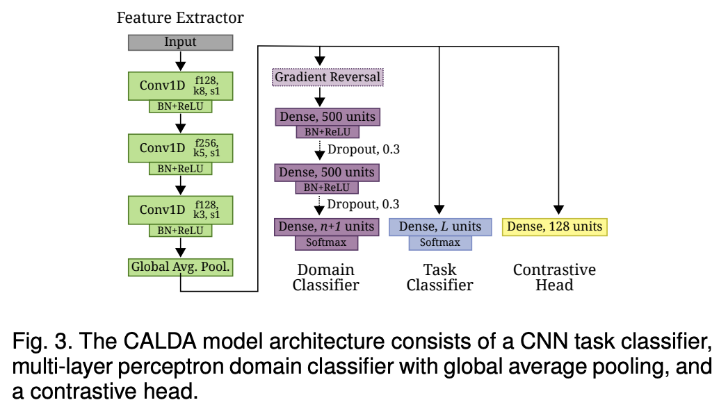
Feature divergence between the train &test

• baseline: Informer
  • 2 encoder layers and 1 decoder layer
  • analyze the features of the first (Layer-1) and the second (Layer-2) encoder layers.
• following the prior work (Pan et al., 2018), we compute the average feature divergence using symmetric KL divergence