(paper 97) Dish-TS; A General Paradigim for Alleviating Distribution for Time Series Forecasting

Dish-TS: A General Paradigim for Alleviating Distribution for Time Series Forecasting (AAAI 2023)

https://arxiv.org/pdf/2302.14829.pdf

https://github.com/weifantt/Dish-TS.

Contents

1. Abstract
2. Introduction
   1. 2 limitations of previous works
   2. Dish_TS
3. Related Work
   1. Models for TSF
   2. Distribution Shift in TSF
4. Problem Formulations
   1. TSF
   2. Distribution Shift in TS
5. Dish-TS
   1. Overview
   2. Dual-Conet Framework
   3. A Simple and Intuitive Instance of Conet
6. Experiment
   1. Experimental Setup
   2. Overall Performance
   3. Comparison with Normalization Methods
   4. Parameters and Model Analysis

Abstract

Problems of existing works towards distribution shift

• mostly limited in the quantification of distribution
• overlook the potential shift between lookback & horizon windows

Distribution shift in TSF into 2 categories

1. INTRA-space shift : input space
2. INTER-space shift : input space & outpt space

Dish-TS

• general neural paradigm for alleviating distribution shift in TSF

• propose the coefficient net (CONET)

  • as a Dual-CONET framework

  • \(\rightarrow\) to separately learn the distribution of input- and output-space

    ( = captures the distribution difference of two spaces 0

1. Introduction

(1) 2 limitations of previous works

1. Distribution quantification for intra-space in TSF is unreliable
   • the empirical statistics are unreliable & limited in expressiveness for representing the true distribution behind the data
   • ex) differ by sampling frequency ( fig 1(b) )

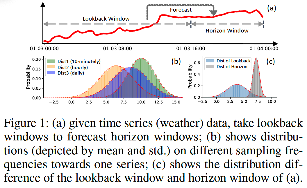
1. Inter-space shift of TSF is neglected

• (preivous works) assume the input-space and output-space follow the same distribution
• RevIN??
  • still limitation … strong assumption that the lookbacks and horizons share the same statistical properties ( = same distn )
  • ex) ( fig 1(c) )

(2) Dish-TS

Dish-TS ( Distribution shift in Time Series )

• model-agnostic
• inspired by RevIN ( normalize & denormalize )

Problem 1) unreliable distribution quantification

Solution 1) coefficient net (CONET)

• to measure the series distribution.

• given any window of series data, maps it into two learnable coefficients
  • (1) level coefficient
  • (2) scaling coefficient
• can be designed as any NN

Problem 2) intra-space shift & inter-space shift

Solution 2) as a DUAL-CONET

• consists of 2 separate CONETS
  • (1) BackCONET
    • coef for INPUT-space ( = lookbacks )
  • (2) HoriCONET
    • Chef for OUTPUT-space ( = horizons )

• distinct distributions for input- and output-space

  \(\rightarrow\) relieves the inter-space shift

2. Related Work

(1) Models for TSF

• pass

(2) Distribution Shift in TSF

Realworld series is changing over time (Akay and Atak 2007)

Adaptive Norm (Ogasawara et al. 2010)

• puts z-score normalization on series by the computed global statistics.

DAIN (Passalis et al. 2019)

• applies NN to adaptively normalize the series.

Adaptive RNNs (Du et al. 2021)

RevIN (Kim et al. 2022)

• instance normalization

Problem 1. ( Except for DAIN .. ) most works still used static statistics or distance function

\(\rightarrow\) limited in expressiveness.

Problem 2. Hardly consider the inter-space shift

• between model input-space and output-space.

3. Problem Formulations

(1) TSF

Notation

• \(x_t\) : value at time-step \(t\)
• input : \(\boldsymbol{x}_{t-L: t}=\left[x_{t-L+1}, \cdots, x_t\right]\)
• output : \(\boldsymbol{x}_{t: t+H}=\left[x_{t+1}, \cdots, x_{t+H}\right]\)
  • \(L\) : the length of lookback windows
  • \(H\) : the length of horizon windows
• \(N\) multivariate time series : \(\left\{x_t^{(1)}, x_t^{(2)}, \cdots, x_t^{(N)}\right\}_{t=1}^T\)
• MTSF task : \(\left(\boldsymbol{x}_{t: t+H}^{(1)}, \cdots, \boldsymbol{x}_{t: t+H}^{(N)}\right)^T=\mathscr{F}_{\Theta}\left(\left(\boldsymbol{x}_{t-L: t}^{(1)}, \cdots, \boldsymbol{x}_{t-L: t}^{(N)}\right)^T\right)\)
  • mapping function \(\mathscr{F}_{\Theta}: \mathbb{R}^{L \times N} \rightarrow \mathbb{R}^{H \times N}\)

(2) Distn shift in TS

a) Intra-space shift

• for any time-step \(u \neq v\), \(\mid d\left(\mathcal{X}_{\text {input }}^{(i)}(u), \mathcal{X}_{\text {input }}^{(i)}(v)\right) \mid >\delta\)
  • \(\delta\) is a small threshold
  • \(d\) is a distance function (e.g., KL divergence)
  • \(\mathcal{X}_{\text {input }}^{(i)}(u)\) and \(\mathcal{X}_{\text {input }}^{(i)}(v)\) : distributions

Most existing works:

• mention distribution shift in series, they mean our called intra-space shift

b) Inter-space shift

• \(\mid d\left(\mathcal{X}_{\text {input }}^{(i)}(u), \mathcal{X}_{\text {output }}^{(i)}(u)\right) \mid >\delta\).

( mostly ignored by current TSF models )

4. Dish-TS

(1) Overview

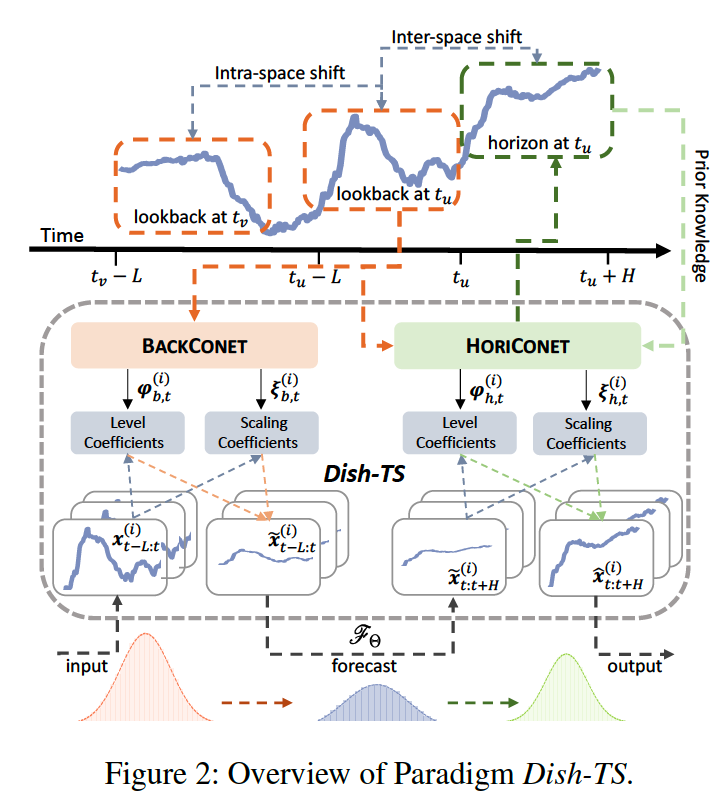
Dual CONET

• transform INPUT
  • via coef obtained from BACKCONET
• transform OUTPUT
  • via coef obtained from HORICONET
  • becomes the forecasting output

(2) Dual-Conet Framework

illustrate how forecasting models are integrated into DualCONET

• by a two-stage normalize-denormalize process.

a) Conet (coefficient net )

\(\boldsymbol{\varphi}, \boldsymbol{\xi}=\operatorname{CONeT}(\boldsymbol{x})\).

• \(\varphi \in \mathbb{R}^1\) : level coefficient
  • overall scale of input series in a window \(\boldsymbol{x} \in \mathbb{R}^L\)
• \(\boldsymbol{\xi} \in \mathbb{R}^1\) : scaling coefficient
  • fluctuation scale of \(\boldsymbol{x}\).

b) Dual-Conet

Goal: to deal with intra-space shift and inter-space shift

\(\begin{aligned} & \boldsymbol{\varphi}_{b, t}^{(i)}, \boldsymbol{\xi}_{b, t}^{(i)}=\operatorname{BACKCONET}\left(\boldsymbol{x}_{t-L: t}^{(i)}\right), i=1, \cdots, N \\ & \boldsymbol{\varphi}_{h, t}^{(i)}, \boldsymbol{\xi}_{h, t}^{(i)}=\operatorname{HoRiCONET}\left(\boldsymbol{x}_{t-L: t}^{(i)}\right), i=1, \cdots, N \end{aligned}\),

• \(\boldsymbol{\varphi}_{b, t}^{(i)}, \boldsymbol{\xi}_{b, t}^{(i)} \in \mathbb{R}^1\) : coefficients for lookbacks
• \(\boldsymbol{\varphi}_{h, t}^{(i)}, \boldsymbol{\xi}_{h, t}^{(i)} \in \mathbb{R}^1\) : coefficients for horizons

\(\rightarrow\) share the same input \(\boldsymbol{x}_{t-L: t}^{(i)}\),

BACKCONET

• aims to approximate distribution \(\mathcal{X}_{\text {input }}^{(i)}\)

HORICONET

• aims to infer (or predict) future distribution \(\mathcal{X}_{\text {output }}^{(i)}\)

c) Integrating Dual-Conet into Forecasting

After acquiring coefficients from Dual-CONET…

\(\rightarrow\) the coefficients can be integrated into any TS

• through a two-stage normalizing-denormalizing process

original forecasting process \(\hat{\boldsymbol{x}}_{t: t+H}^{(i)}=\mathscr{F}_{\Theta}\left(\boldsymbol{x}_{t-L: t}^{(i)}\right)\) is rewritten as:

• \(\hat{\boldsymbol{x}}_{t: t+H}^{(i)}=\boldsymbol{\xi}_{h, t}^{(i)} \mathscr{F}_{\Theta}\left(\frac{1}{\boldsymbol{\xi}_{b, t}^{(i)}}\left(\boldsymbol{x}_{t-L: t}^{(i)}-\boldsymbol{\varphi}_{b, t}^{(i)}\right)\right)+\boldsymbol{\varphi}_{h, t}^{(i)}\).

(3) A Simple and Intuitive Instance of Conet

Flexibility of Dish-TS comes from the specific CONET design

• which could be any neural architectures for different modeling capacity.

Most intuitive way : FC layer

• Input : multivariate input \(\left\{\boldsymbol{x}_{t-L: t}^{(i)}\right\}_{i=1}^N\),
• FC layer : \(\mathbf{v}_b^{\ell}, \mathbf{v}_h^{\ell} \in \mathbb{R}^{L * N}\)
• ( consider \(\ell=1\) for simplicity )
  • \(\boldsymbol{\varphi}_{b, t}^{(i)}=\sigma\left(\sum_{\tau=1}^{\operatorname{dim}\left(\mathbf{v}_{b, i}^{\ell}\right)} \mathbf{v}_{b, i \tau}^{\ell} x_{\tau-L+t}^{(i)}\right)\).
  • \(\varphi_{h, t}^{(i)}=\sigma\left(\sum_{\tau=1}^{\operatorname{dim}\left(\mathbf{v}_{h, i}^{\ell}\right)} \mathbf{v}_{h, i \tau}^{\ell} x_{\tau-L+t}^{(i)}\right)\).
    • \(\sigma\) : leaky ReLU

Scaling coefficients:

• \(\boldsymbol{\xi}_{b, t}^{(i)}=\sqrt{\mathbb{E}\left(x_t^{(i)}-\boldsymbol{\varphi}_{b, t}^{(i)}\right)^2}\).

• \(\boldsymbol{\xi}_{h, t}^{(i)}=\sqrt{\mathbb{E}\left(x_t^{(i)}-\varphi_{h, t}^{(i)}\right)^2}\).

  • can be seen as the average deviation of \(\boldsymbol{x}_{t-L: t}^{(i)}\) with regard to \(\boldsymbol{\varphi}_{b, t}^{(i)}\) and \(\boldsymbol{\varphi}_{h, t}^{(i)}\).

5. Experiment

(1) Experimental Setup

a) Dataset

• Electricity
• ETT (ETTh1, ETTm2)
• Weather
• Illness

b) Evaluation

without data normalization or scaling

• evaluations are on original data

  \(\rightarrow\) thus the reported metrics are scaled for readability.

c) Implementation

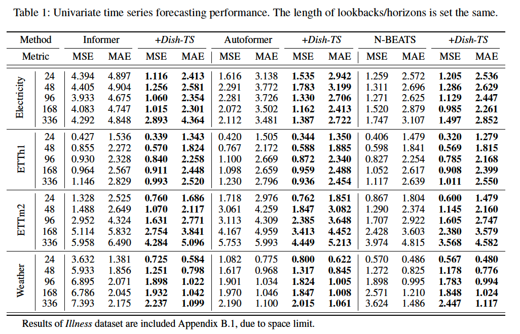
• lookback length = horizon length
  • except for Illness) from 24 to 336

d) Baselines

3 SOTA models

• Informer
• Autoformer
• N-Beats

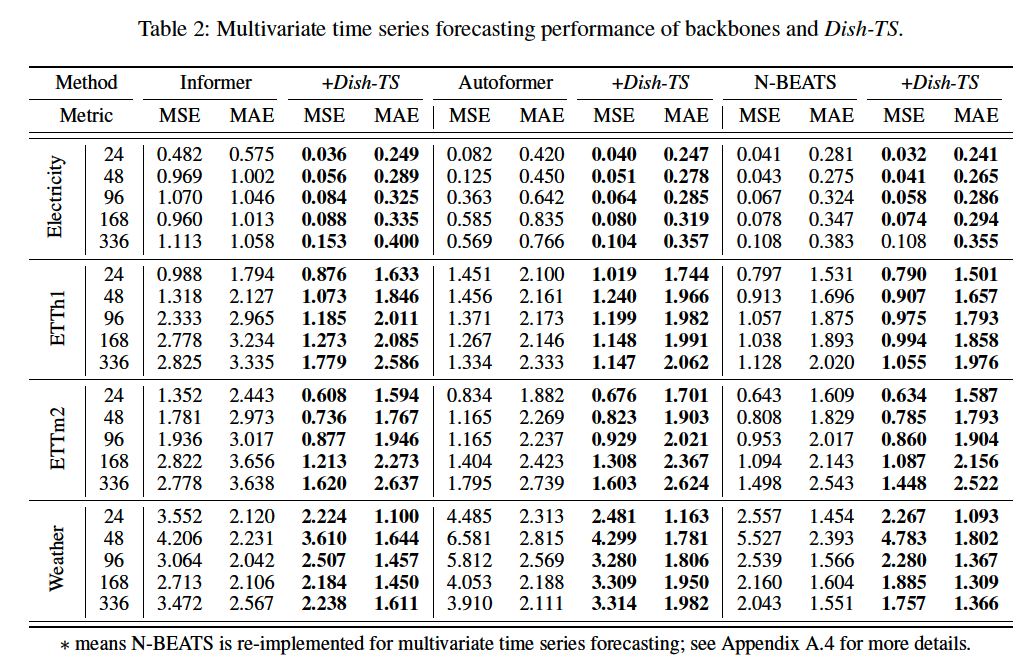
(2) Overall Performance

a) UTS forecasting

b) MTS forecasting

(3) Comparison with Normalization Methods

compare with RevIN (Kim et al. 2022)

( don’t consider AdaRNN (Du et al. 2021), because it is not compatible for fair comparisons )

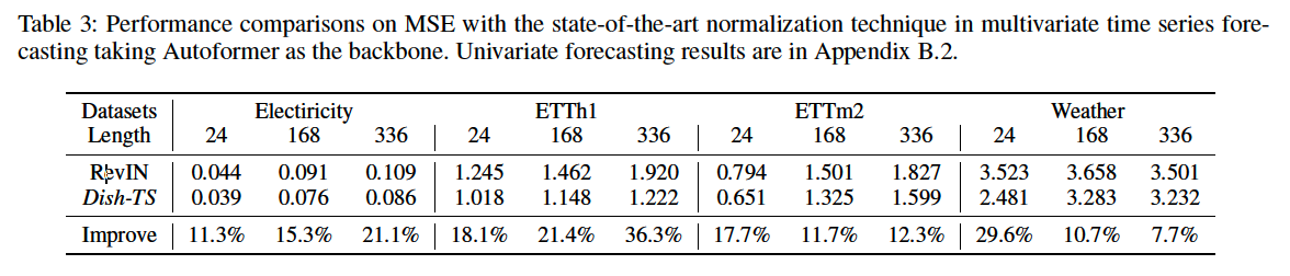
A potential reason ?

\(\rightarrow\) consideration towards both intra-space shift and inter-space shift.

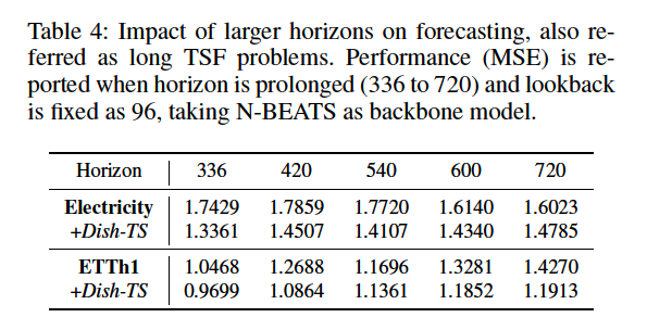
(4) Parameters and Model Analysis

a) Horizon (\(H\)) Analysis

Effect of using larger horizons ( = LTSF )

• fix \(L = 96\)

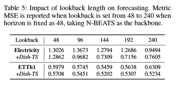
b) Lookback (\(L\)) Analysis

Effect of using larger input length

• fix \(H = 48\)

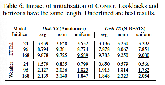
c) Conet Initialization

Initialization for FC layer : \(\mathbf{v}_b^{\ell}, \mathbf{v}_h^{\ell} \in \mathbb{R}^{L * N}\)

• avg : 1
• norm : \(N(0,1)\)
• uniform : \(U(0,1)\)

Result: do not use norm !

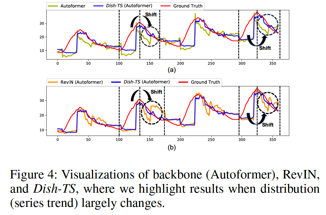
d) Visualizations