(paper) Deep and Confident Prediction for Time Series at Uber

Deep and Confident Prediction for Time Series at Uber (2017)

Contents

1. Abstract
2. Introduction
3. Related Works
   1. BNN
4. Method
   1. Prediction Uncertainty
   2. Model Design

0. Abstract

Reliable Uncertainty Estimation

• propose a novel end-to-end Bayesian Deep Model

1. Introduction

estimating uncertainty in TS prediction!

quantify the prediction uncertainty, using BNN, which is further used for large-scale anomaly detection

Prediction Uncertainty

• 1) model uncertainty ( = epistemic uncertainty )
  • can be reduced, as more samples being collected
• 2) inherent noise
  • captures the uncertainty in the data generation process
• 3) model misspecification
  • test data distn \(\neq\) train data distn

Propose a principled solution to incorporate this uncertainty using an encoder-decoder framework

Contributions (Summary)

• generic & scalable uncertainty estimation implementation
• quantifies the prediction uncertainty from 3 sources
• motivates a real-world anomaly detection

2. Related Works

2-1. BNN

this paper is inspired by MCDO (Monte Carlo Drop Out)

• stochastic dropouts are applied after each hidden layer
• model output = random sample, generated from posterior predictive distn
• model uncertainty can be estimated by sample variance of the model prediction

3. Method

trained NN : \(f^{\hat{W}}(\cdot)\)

new sample : \(x^{*}\)

\(\rightarrow\) goal : evaluate the uncertainty of the model prediction, \(\hat{y}^{*}=f^{\hat{W}}\left(x^{*}\right) .\)

quantify the prediction standard error, \(\eta\),

so that an approximate \(\alpha\)-level prediction interval = \(\left[\hat{y}^{*}-z_{\alpha / 2} \eta, \hat{y}^{*}+z_{\alpha / 2} \eta\right]\).

(1) Prediction Uncertainty

• NN : \(f^{W}(\cdot)\)…. gaussian prior : \(W \sim N(0, I)\)

• data generating distribution : \(p\left(y \mid f^{W}(x)\right)\)

  • ex) for regression : \(y \mid W \sim N\left(f^{W}(x), \sigma^{2}\right)\)

• dataset

  • set of \(N\) observations \(X=\left\{x_{1}, \ldots, x_{N}\right\}\) and \(Y=\left\{y_{1}, \ldots, y_{N}\right\}\)

• Bayesian inference : finding the posterior distribution over model parameters \(p(W \mid X, Y)\).

• prediction distribution :

  • obtained by marginalizing out the posterior distribution
  • \(p\left(y^{*} \mid x^{*}\right)=\int_{W} p\left(y^{*} \mid f^{W}\left(x^{*}\right)\right) p(W \mid X, Y) d W\).

• variance of the prediction distn

  • decomposed into…

    \(\begin{aligned} \operatorname{Var}\left(y^{*} \mid x^{*}\right) &=\operatorname{Var}\left[\mathbb{E}\left(y^{*} \mid W, x^{*}\right)\right]+\mathbb{E}\left[\operatorname{Var}\left(y^{*} \mid W, x^{*}\right)\right] \\ &=\operatorname{Var}\left(f^{W}\left(x^{*}\right)\right)+\sigma^{2} \end{aligned}\).

  • 2 terms :

    • 1) \(\operatorname{Var}\left(f^{W}\left(x^{*}\right)\right)\) : model uncertainty
    • 2) \(\sigma^{2}\) : inherent noise

• this paper considers COMBINATION of 3 SOURCES

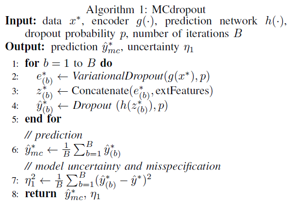
(a) Model Uncertainty

• stochastic dropouts at each layer

• randomly dropout each hidden unit with certain probability \(p\)

• stochastic feedforward is repeated \(B\) times \(\rightarrow\) \(\left\{\hat{y}_{(1)}^{*}, \ldots, \hat{y}_{(B)}^{*}\right\}\).

• Model uncertainty : can be approximated by the sample variance

  • \(\widehat{\operatorname{Var}}\left(f^{W}\left(x^{*}\right)\right)=\frac{1}{B} \sum_{b=1}^{B}\left(\hat{y}_{(b)}^{*}-\overline{\hat{y}}^{*}\right)^{2}\).

    where \(\overline{\hat{y}}^{*}=\frac{1}{B} \sum_{b=1}^{B} \hat{y}_{(b)}^{*} \quad[13]\)

(b) Model misspecification

• use encoder & decoder
• [idea] train an encoder that extracts the representative features from a time series & decode it

• measure the distance between test cases & training samples in the embedded space

• How to incorporate this uncertainty in variance calculation?
  • connecting encoder \(g(\cdot)\) with prediction network \(h(\cdot)\)
  • treat them as one network ( \(f = h(g(\cdot))\) )

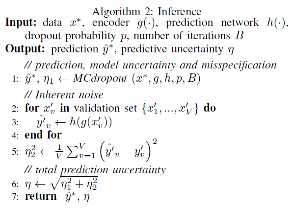
(c) Inherent noise

• inherent noise level = \(\sigma^2\)

• propose a simple & adaptive approach, that estimates the noise level

  via the sum of squares, evaluated on an independent HELD-OUT VALIDATION set

  ( \(X^{\prime}=\left\{x_{1}^{\prime}, \ldots, x_{V}^{\prime}\right\}, Y^{\prime}=\left\{y_{1}^{\prime}, \ldots, y_{V}^{\prime}\right\}\) )

• estimate \(\sigma^{2}\) via \(\hat{\sigma}^{2}=\frac{1}{V} \sum_{v=1}^{V}\left(y_{v}^{\prime}-f^{\hat{W}}\left(x_{v}^{\prime}\right)\right)^{2}\)

Final inference algorithm :

• combine inherent noise estimation with MC dropout

(2) Model Design

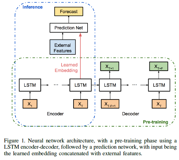
• part 1) encoder-decoder framework
• part 2) prediction network

(a) Encoder-decoder

conduct a pre-training step to fit an encoder ( = 2-layer LSTM )

Notation

• univariate time series \(\left\{x_{t}\right\}_{t}\)
• encoder reads in the first \(T\) timestamps \(\left\{x_{1}, \ldots, x_{T}\right\}\)
• decoder constructs the following \(F\) timestamps \(\left\{x_{T+1}, \ldots, x_{T+F}\right\}\) with guidance from \(\left\{x_{T-F+1}, \ldots, x_{T}\right\}\)

(b) Prediction network

when external features are available

\(\rightarrow\) concatenated to the embedding vector

(c) Inference

inference stage involves only encoder & prediction network

prediction uncertainty \(\eta\) contains 2 terms

• 1) model uncertainty & misspecification uncertainty
• 2) inherent noise

Finally, approximate \(\alpha\) level prediction interval is constructed!

\(\left[\hat{y}^{*}-z_{\alpha / 2} \eta, \hat{y}^{*}+z_{\alpha / 2} \eta\right]\).