(paper) GP-VAE ; Deep Probabilistic Time Series Imputation

GP-VAE ; Deep Probabilistic Time Series Imputation (2020)

Contents

1. Abstract

2. Introduction

3. Related Work

4. Model

   1. Problem Setting & Notation

   2. Generative model ( \(z \rightarrow x\) )

   3. Inference model ( \(x \rightarrow z\) )

0. Abstract

MTS with missing values!

\(\rightarrow\) DL? classical data imputation methods?

Propose a new Deep sequential latent variable model for

• 1) dimensionality reduction
• 2) data imputation

Simple & interpretable assumption

• high dim time series data \(\rightarrow\) low dim representation, which evolves smoothly according to GP
• non-linear dim reduction by VAE

1. Introduction

MTS (Multivariate Time Series)

• multiple correlated univariate time series(=channel)

• 2 ways of imputation

  • 1) exploiting temporal correlations WITHIN each channel
  • 2) exploiting temporal correlations ACROSS channels

  \(\rightarrow\) should consider BOTH ( current algorithms : only ONE )

Previous Works for MTS

1. Time-tested statistical methods ( ex) GP )

• works well for complete data
• not applicable when features are missing

1. Classical methods for time series imputation

• interaction BETWEEN channels (X)

1. Recent works

• non-linear dim reduction using VAES
• sharing statistical strength across time (X)

Proposal

• combine “non-linear dimm reduction” + “expressive time-series model”

• by jointly learning a mapping from data space (missing O) \(\rightarrow\) latent space (missing X)

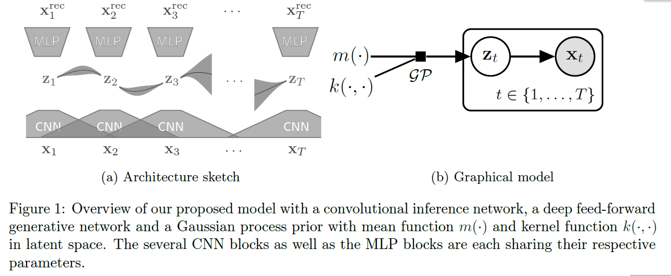
• proposes an architecture that use..
  • 1) VAE to map missing data time series into latent space
  • 2) GP to model low-dimensional dynamics

Contributions

• 1) propose VAE architecture for MTS imputation with a GP prior in the latent space to capture temporal dynamics
• 2) Efficient Inference ( Structued VI )
• 3) Benchmarking on real-world data

2. Related Work

a) Classical statistical approaches

• mean imputation, forward imputation
• simple / efficient & interpretable
• EM algorithm ( often require additional modeling assumptions )

b) Bayesian methods

• estimate likelihoods/uncertainties ( ex. GP )
• limited scalability & challenges in designing kernels that are robust to missing values

c) Deep Learning techniques

• VAEs & GANS
  • VAEs : tractable likelihood
  • GANS : intractable
• none of these explicitly take temporal dynamics into account

d) HI-VAE

• deals with missing data by defining an ELBO, whose reconstruction error only “sums over the observed part”

• (for inference) incomplete data = zero imputation

  \(\rightarrow\) unavoidable bias

• (ours vs HI-VAE) temporal information O/X

  • HI-VAE) not formulated for sequential data
  • ours) formulated for sequential data

e) Deep Learning for time series imputation

• do not model temporal dynamics when dealing with missing values

3. Model

propose novel architecture for “missing value imputation”

Main idea

• 1) embed the data into latent space
• 2) model the temporal dynamics in this latent space
  • capture correlations & use them to reconstruct missing values
  • GP prior : make temporal dynamics smoother & explainable

(1) Problem Setting & Notation

Notation

• MTS data : \(\mathbf{X} \in \mathbb{R}^{T \times d}\)

  ( \(T\) data points : \(\mathbf{x}_{t}=\left[x_{t 1}, \ldots, x_{t j}, \ldots, x_{t d}\right]^{\top} \in \mathbb{R}^{d}\) )

  ( any number of these data features \(x_{t j}\) can be missing )

• \(T\) consecutive time points \(\tau=\left[\tau_{1}, \ldots, \tau_{T}\right]^{\top}\)

observed & unobserved

• \(\mathrm{x}_{t}^{o}:=\left[x_{t j} \mid x_{t j}\right.\) is observed]
• \(\mathbf{x}_{t}^{m}:=\left[x_{t j} \mid x_{t j}\right.\) is missing \(]\)

Missing value imputation

• estimating the true values of the missing features \(\mathbf{X}^{m}:=\left[\mathbf{x}_{t}^{m}\right]_{1: T}\) given the observed features \(\mathbf{X}^{o}:=\left[\mathrm{x}_{t}^{o}\right]_{1: T} .\)

• many methods assume the different data points to be independent

  \(\rightarrow\) inference problem reduces to \(T\) separate problems of estimating \(p\left(\mathbf{x}_{t}^{m} \mid \mathbf{x}_{t}^{o}\right)\)

• ( for time series )

  this independence assumption is not satisfied

  \(\rightarrow\) more complex estimation problem of \(p\left(\mathbf{x}_{t}^{m} \mid \mathbf{x}_{1: T}^{o}\right)\).

(2) Generative model ( \(z \rightarrow x\) )

• reducing data (with missing) into representations (without missing)
• modeling dynamics in this low-dim representation using Gaussian Process
• GP time complexity : \(O(n^3)\)
  • worser when missing values!
  • option 1 : fill with zero
    • problem : make 2 data points with different missingness pattern look very dissimilar, when in fact they are close
  • option 2 : treat every channel of MTS separately
    • problem : ignores valuable correlation across channels

• overcome these problems by defining a suitable GP kernel in the data space with missing observations,

  by instead “applying the GP” in the latent space of VAE

  • assign latent variable \(\mathrm{z}_{t} \in \mathbb{R}^{k}\) for every \(\mathrm{x}_{t}\)
  • model temporal correlations in this reduced representation \(\mathbf{z}(\tau) \sim \mathcal{G} \mathcal{P}\left(m_{z}(\cdot), k_{z}(\cdot, \cdot)\right)\)

• kernel

  • Rational Quadratic kernel ( = infinite mixture of RBF kernels )

    \(\int p(\lambda \mid \alpha, \beta) k_{R B F}(r \mid \lambda) d \lambda \propto\left(1+\frac{r^{2}}{2 \alpha \beta^{-1}}\right)^{-\alpha}\).

  • Cauchy kernel ( For \(\alpha=1\) and \(l^{2}=2 \beta^{-1}\), it red Cauchy kernel)

    \(k_{C a u}\left(\tau, \tau^{\prime}\right)=\sigma^{2}\left(1+\frac{\left(\tau-\tau^{\prime}\right)^{2}}{l^{2}}\right)^{-1}\).

• generation :

  \(p_{\theta}\left(\mathbf{x}_{t} \mid \mathbf{z}_{t}\right)=\mathcal{N}\left(g_{\theta}\left(\mathbf{z}_{t}\right), \sigma^{2} \mathbf{I}\right)\).

(3) Inference model ( \(x \rightarrow z\) )

• interested in posterior, \(p\left(\mathbf{z}_{1: T} \mid \mathbf{x}_{1: T}\right)\)

• use variational inference

• approximate true posterior \(p\left(\mathbf{z}_{1: T} \mid \mathbf{x}_{1: T}\right)\) with multivariate Gaussian \(q\left(\mathbf{z}_{1: T, j} \mid \mathbf{x}_{1: T}^{o}\right)\)

  \(q\left(\mathbf{z}_{1: T, j} \mid \mathbf{x}_{1: T}^{o}\right)=\mathcal{N}\left(\mathbf{m}_{j}, \mathbf{\Lambda}_{j}^{-1}\right)\).

  • precision matrix : parameterized in terms of a product of “bidiagonal matrices”

    \(\boldsymbol{\Lambda}_{j}:=\mathbf{B}_{j}^{\top} \mathbf{B}_{j}, \text { with }\left\{\mathbf{B}_{j}\right\}_{t t^{\prime}}= \begin{cases}b_{t t^{\prime}}^{j} & \text { if } t^{\prime} \in\{t, t+1\} \\ 0 & \text { otherwise }\end{cases}\).