
Handling Incomplete Heterogeneous Data using VAEs (2020)
Contents
- Abstract
- Introduction
- Problem Statement
- Generalizing VAEs for H & I data
- Handling Incomplete data
- Handling heterogeneous data
- Summary
- HI-VAE (Heterogeneous-Incomplete VAE)
0. Abstract
VAEs : efficient & accurate for capturing “latent structure”
VAE 문제점 : can not handle data that are…
- 1) heterogeneous ( continuous + discrete )
- 2) incomplete ( missing data )
Propose “HI-VAE”
- suitable for fitting “incomplete & heterogeneous” data
1. Introduction
underlying latent structure
\(\rightarrow\) allow us to better understand the data
Deep generative models
- highly flexible & expressive unsupervised methods
-
able to capture “latent structure” of “complex high-dim data”
- ex) VAEs & GANs
\(\rightarrow\) current DGMs focus on “HOMOgeneous data” collections
( Not many attention to “HETEROgeneous data”)
This paper :
- present a general framework for VAEs that effectively incorporates incomplete data & heterogeneous observations
Features
- 1) GENERATIVE model that handles both mixed (1) numerical & (2) nominal
- 2) handles MCAR (Missing Data Completely at Random)
- 3) data-normalization input/output layer
- 4) ELBO used to optimized generative/recognition models
2. Problem Statement
HETEROgeneous dataset : \(N\) objects & \(D\) attributes
- dataset : \(\mathbf{x}_{n}=\left[x_{n 1}, \ldots, x_{n D}\right]\)
[ Data type ]
Numerical variables:
- Real-valued data … \(x_{n d} \in \mathbb{R}\).
- Positive real-valued data … \(x_{n d} \in \mathbb{R}^{+}\).
- (Discrete) count data … \(x_{n d} \in\{1, \ldots, \infty\}\).
Nominal variables:
- Categorical data … \(x_{n d} \in\{\) ‘blue’, ‘red’, ‘black’ \(\}\).
- Ordinal data … \(x_{n d} \in\{\) ‘never’, ‘sometimes’, ‘often’, ‘usually’, ‘always’ \(\}\).
[ Missingness ]
- \(\mathcal{O}_{n}\) : observed data index
- \(\mathcal{M}_{n}\) : missing data index
3. Generalizing VAEs for H & I data
( H data : Heterogeneous data )
( I data : Incomplete data )
(1) Handling Incomplete data
-
generator (decoder) & recognition (encoder)
-
factorization for the decoder : \(p\left(\mathbf{x}_{n}, \mathbf{z}_{n}\right)=p\left(\mathbf{z}_{n}\right) \prod_{d} p\left(x_{n d} \mid \mathbf{z}_{n}\right)\).
- \(\mathbf{z}_{n} \in \mathbb{R}^{K}\) : latent vector
- \(p\left(\mathbf{z}_{n}\right)=\mathcal{N}\left(\mathbf{z}_{n} \mid \mathbf{0}, \mathbf{I}_{K}\right)\).
- makes it easy to marginalize out the missing attributes
-
likelihood : \(p\left(x_{n d} \mid \mathbf{z}_{n}\right)\)
-
parameters : \(\gamma_{n d}=\mathbf{h}_{d}\left(\mathbf{z}_{n}\right)\)
( \(\mathbf{h}_{d}\left(\mathbf{z}_{n}\right)\) : DNN that transforms the \(\mathbf{z}_{n}\) into parameters \(\gamma_{n d}\) )
-
-
factorization of likelihood :
- missing & observed
- \(p\left(\mathrm{x}_{n} \mid \mathbf{z}_{n}\right)=\prod_{d \in \mathcal{O}_{n}} p\left(x_{n d} \mid \mathbf{z}_{n}\right) \prod_{d \in \mathcal{M}_{n}} p\left(x_{n d} \mid \mathbf{z}_{n}\right)\).
- recognition model : \(q\left(\mathbf{z}_{n}, \mathbf{x}_{n}^{m} \mid \mathbf{x}_{n}^{o}\right)\)
-
factorization of recognition model :
- \(q\left(\mathbf{z}_{n}, \mathbf{x}_{n}^{m} \mid \mathbf{x}_{n}^{o}\right)=q\left(\mathbf{z}_{n} \mid \mathbf{x}_{n}^{o}\right) \prod_{d \in \mathcal{M}_{n}} p\left(x_{n d} \mid \mathbf{z}_{n}\right)\).
Recognition models (=encoder) for incomplete data
- propose “input drop-out recognition distribution”
- \(q\left(\mathbf{z}_{n} \mid \mathbf{x}_{n}^{o}\right)=\mathcal{N}\left(\mathbf{z}_{n} \mid \boldsymbol{\mu}_{q}\left(\tilde{\mathbf{x}}_{n}\right), \mathbf{\Sigma}_{q}\left(\tilde{\mathbf{x}}_{n}\right)\right)\).
- missing dimensions are replaced by zero
- \(\mu_{q}\left(\tilde{\mathbf{x}}_{n}\right)\) and \(\Sigma_{q}\left(\tilde{\mathbf{x}}_{n}\right)\) are parametrized DNNs with input \(\tilde{\mathbf{x}}_{n}\)
- VAE for incomplete data
- \(p\left(\mathrm{x}_{n}^{m} \mid \mathrm{x}_{n}^{o}\right) \approx \int p\left(\mathrm{x}_{n}^{m} \mid \mathbf{z}_{n}\right) q\left(\mathbf{z}_{n} \mid \mathbf{x}_{n}^{o}\right) d \mathbf{z}_{n}\).
(2) Handling heterogeneous data
- choose appropriate likelihood function, depending on data type
-
Real-valued : \(p\left(x_{n d} \mid \gamma_{n d}\right)=\mathcal{N}\left(x_{n d} \mid \mu_{d}\left(\mathbf{z}_{n}\right), \sigma_{d}^{2}\left(\mathbf{z}_{n}\right)\right)\)
-
Positive real-valued : \(p\left(x_{n d} \mid \gamma_{n d}\right)=\log \mathcal{N}\left(x_{n d} \mid \mu_{d}\left(\mathbf{z}_{n}\right), \sigma_{d}^{2}\left(\mathbf{z}_{n}\right)\right)\)
-
Count : \(p\left(x_{n d} \mid \gamma_{n d}\right)=\operatorname{Poiss}\left(x_{n d} \mid \lambda_{d}\left(\mathbf{z}_{n}\right)\right)=\frac{\left(\lambda_{d}\left(\mathbf{z}_{n}\right)\right)^{x_{n d}} \exp \left(-\lambda_{d}\left(\mathbf{z}_{n}\right)\right)}{x_{n d} !}\)
-
Categorical : \(p\left(x_{n d}=r \mid \gamma_{n d}\right)=\frac{\exp \left(-h_{d r}\left(\mathbf{z}_{n}\right)\right)}{\sum_{q=1}^{R} \exp \left(-h_{d q}\left(\mathbf{z}_{n}\right)\right)}\).
-
Ordinal : \(p\left(x_{n d}=r \mid \gamma_{n d}\right)=p\left(x_{n d} \leq r \mid \gamma_{n d}\right)-p\left(x_{n d} \leq r-1 \mid \gamma_{n d}\right)\)
with \(p\left(x_{n d} \leq r \mid \mathbf{z}_{n}\right)=\frac{1}{1+\exp \left(-\left(\theta_{r}\left(\mathbf{z}_{n}\right)-h_{d}\left(\mathbf{z}_{n}\right)\right)\right)}\)
(3) Summary
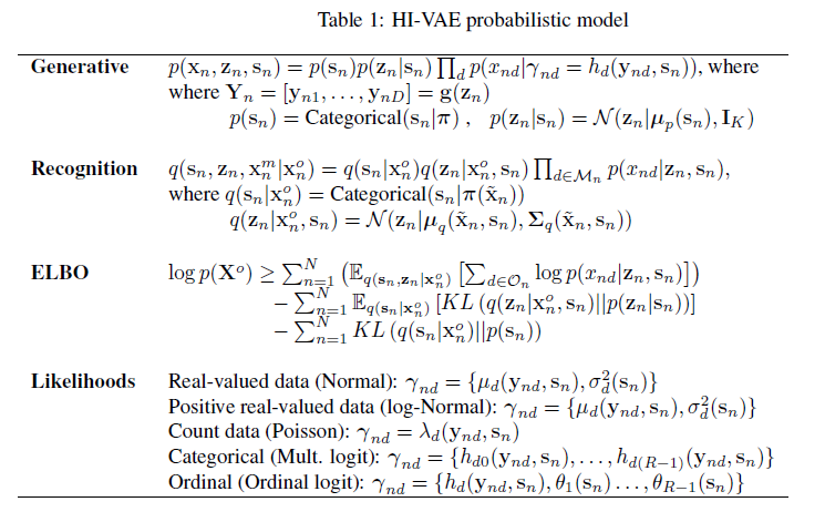
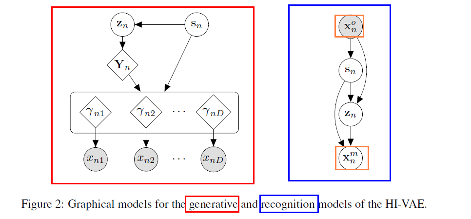
4. HI-VAE (Heterogeneous-Incomplete VAE)
generative model that fully factorizes for every heterogeneous dimension in the data
\(\rightarrow\) loses the properties of AMORTIZED generative models
(1) propose Gaussian Mixture prior
- \(p\left(\mathbf{s}_{n}\right) =\text { Categorical }\left(\mathbf{s}_{n} \mid \boldsymbol{\pi}\right)\).
- \(p\left(\mathbf{z}_{n} \mid \mathbf{s}_{n}\right) =\mathcal{N}\left(\mathbf{z}_{n} \mid \boldsymbol{\mu}_{p}\left(\mathbf{s}_{n}\right), \mathbf{I}_{K}\right)\).
- \(\mathrm{s}_{n}\) is a one-hot encoding vector representing the component in the mixture
- assume \(\pi_{\ell}=1 / L\) ( uniform )
(2) propose hierarchical structure
-
allows different attributes to share network parameter
( amortize generative model )
(3) introduce an “intermediate homogeneous representation” of the data
- \(\mathbf{Y}=\left[\mathbf{y}_{n 1}, \ldots, \mathbf{y}_{n D}\right]\).
- jointly generated by single DNN with input \(\mathbf{z}_{n}\), \(\mathrm{g}\left(\mathbf{z}_{n}\right)\)
(4) likelihood params of each atttribute \(d\) = output of DNN
- \(p\left(x_{n d} \mid \gamma_{n d}=\mathbf{h}_{d}\left(\mathbf{y}_{n d}, \mathbf{s}_{n}\right)\right)\).
(5) Recognition model : \(q\left(\mathrm{~s}_{n} \mid \mathrm{x}_{n}^{o}\right)\)
-
categorical distn with param vector \(\pi\)
-
output of DNN with input \(\tilde{\mathbf{x}}_{n}\) & softmax
-
factorization
\(q\left(\mathbf{s}_{n}, \mathbf{z}_{n}, \mathbf{x}_{n}^{m} \mid \mathbf{x}_{n}^{o}\right)=q\left(\mathbf{s}_{n} \mid \mathbf{x}_{n}^{o}\right) q\left(\mathbf{z}_{n} \mid \mathbf{x}_{n}^{o}, \mathbf{s}_{n}\right) \prod_{d \in \mathcal{M}_{n}} p\left(x_{n d} \mid \mathbf{z}_{n}, \mathbf{s}_{n}\right)\).
.