
Probabilistic Time Series Forecasting with Implicit Quantile Networks (2021)
Contents
- Abstract
- Introduction
- Background
- Quantile Regression
- CRPS
- Forecasting with IQN
0. Abstract
propose general method for probabilistic time-series forcasting
combine (1) & (2)
-
(1) autoregressive RNN
\(\rightarrow\) to model “temporal dynamics”
-
(2) Implicit Quantile Networks
\(\rightarrow\) to learn a “large class of distn” over a time-series target
This method is favorable in terms of…
- point-wise prediction accuracy
- estimating the underlying temporal distn
1. Introduction
[ Traditional ]
-
univariate point forecast
-
require to learn “one model per individual t.s”
( not scale for large data )
[ Deep Learning ]
- RNN, LSTM…
- main advantages
- end-to-end
- ease of incorporating exogenous covariates
- automatic feature extractions
Desirable to make a probabilistic output
\(\rightarrow\) provide uncertainty bounds!
- method 1) model the data distn explicitly
- method 2) Bayesian NN
Propose IQN-RNN
-
“DL-based univariate t.s method, that learns an implicit distn over outputs”
-
does not make any assumption on the underlying distn
-
probabilistic output is generated by IQN
& trained by minimizing CRPS (=Continuous Ranked Probability Score )
Contributions
- model data distn using IQNs
- model t.s via autoregressive RNN
2. Background
(1) Quantile Regression
Quantile function corresponding to c.d.f \(F: \mathbb{R} \rightarrow[0,1]\)
- \(Q(\tau)=\inf \{x \in \mathbb{R}: \tau \leq F(x)\}\).
- For continuous and strictly monotonic c.d.f. \(Q=F^{-1}\)
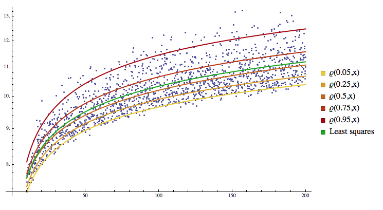
Minimize quantile loss :
-
\(L_{\tau}(y, \hat{y})=\tau(y-\hat{y})_{+}+(1-\tau)(\hat{y}-y)_{+},\).
( where ()\(_{+}\) is ReLU )
(2) CRPS
Continuous Ranked Probability Score
-
described by a c.d.f. \(F\) given the observation \(y\) :
\(\operatorname{CRPS}(F, y)=\int_{-\infty}^{\infty}(F(x)-\mathbb{1}\{y \leq x\})^{2} d x\).
-
can be rewritten as… (using quantile loss ) :
\(\operatorname{CRPS}(F, y)=2 \int_{0}^{1} L_{\tau}(y, Q(\tau)) d \tau\).
3. Forecasting with IQN
in univariate time series setting…
- forecast \(\left(y_{T-h}, y_{T-h+1}, \ldots, y_{T}\right)\)
- with \(y=\left(y_{0}, y_{1}, \ldots, y_{T}\right)\)
Notation
- \(\tau_{0}=\mathbb{P}\left[Y_{0} \leq y_{0}\right]\).
- \(\tau_{t}=\mathbb{P}[Y_{t} \leq y_{t} \mid Y_{0} \leq \left.y_{0}, \ldots, Y_{t-1} \leq y_{t-1}\right]\).
\(\rightarrow\) rewrite \(y\) as …
- \(\left(F_{Y_{0}}^{-1}\left(\tau_{0}\right), F_{Y_{1} \mid Y_{0}}^{-1}\left(\tau_{1}\right), \ldots, F_{Y_{T} \mid Y_{0}, \ldots, Y_{T}}^{-1}\left(\tau_{T}\right)\right)\).
Probabilistic Time Series Forecasting
-
unique function \(g\) can represent distn of all \(Y_t\),
given \(X_t\) & previous observation \(y_0,...y_{t-1}\)
-
IQN 사용 시, 위의 두 정보 외에도 \(\tau_t\)를 사용!
- mapping from \(\tau_{t} \sim \mathrm{U}([0,1])\) to \(y_{t}\)
IQN-RNN
- learn \(y_{t}=g\left(X_{t}, \tau_{t}, y_{0}, y_{1}, \ldots, y_{t-1}\right)\) ….. for \(t \in [T-h,T]\)
-
can be written as \(q \circ\left[\psi_{t} \odot(1+\phi)\right]\)
-
Notation
-
\(\odot\) : Hadamard element-wise product
-
\(X_{t}\) : (typically) time-dependent features…. known for all time steps
-
\(\psi_{t}\) : state of an RNN
( takes concat(\(X_{t}, y_{t-1},\psi_{t-1})\) as input )
-
\(\phi\) : embeds \(\tau_{t}\)
( \(\phi\left(\tau_{t}\right)=\operatorname{ReLU}\left(\sum_{i=0}^{n-1} \cos \left(\pi i \tau_{t}\right) w_{i}+b_{i}\right)\) )
-
\(q\) : additional generator layer
-
(a) Training
-
step 1) quantiles are sampled
( for each observation / at each time step )
-
step 2) passed to both network & quantile loss
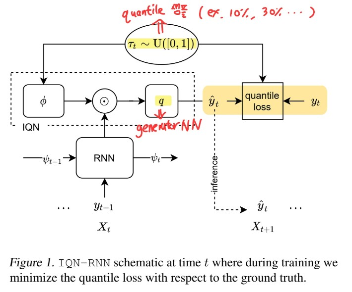
(b) Inference
-
step 1) quantiles are sampled
( for each observation / at each time step )
-
step 2) passed to both network