
N-Beats : Neural Basis Expansion Analysis for Interpretable Time Series Forecasting (2020)
Contents
- Abstract
- Introduction
- Problem Statement
- N-Beats
- Basic Block
- Doubly Residual Stacking
- Interpretability
- Ensemble
0. Abstract
focus on solving UNIVARIATE time series POINT forecasting problem using DL
propose architecture based on…
- 1) backward & forward residual links
- 2) very deep stack of FC layers
Desired Properties
- 1) interpretable
- 2) applicable without modification to a wide array of target domains
- 3) fast to train
1. Introduction
Contributions
- Deep Neural Architecture
- Interpretable DL for time series
2. Problem Statement
Problem
- univariate point forecasting problem
Notation
- length- \(H\) forecast horizon
- length- \(T\) observed series history \(\left[y_{1}, \ldots, y_{T}\right] \in \mathbb{R}^{T}\)
- lookback window of length \(t \leq T\) ( ends with \(y_T\) )
- \(\mathbf{x} \in \mathbb{R}^{t}=\left[y_{T-t+1}, \ldots, y_{T}\right]\).
- \(\widehat{\mathbf{y}}\) : forecast of \(\mathbf{y}\)
Task
- predict \(\mathbf{y} \in \mathbb{R}^{H}=\left[y_{T+1}, y_{T+2}, \ldots, y_{T+H}\right] .\)
Forecasting performance
\[\begin{aligned} \text { SMAPE } &=\frac{200}{H} \sum_{i=1}^{H} \frac{ \mid y_{T+i}-\widehat{y}_{T+i} \mid }{ \mid y_{T+i} \mid + \mid \widehat{y}_{T+i} \mid }, \quad \text { MAPE }=\frac{100}{H} \sum_{i=1}^{H} \frac{ \mid y_{T+i}-\widehat{y}_{T+i} \mid }{ \mid y_{T+i} \mid } \\ \operatorname{MASE} &=\frac{1}{H} \sum_{i=1}^{H} \frac{ \mid y_{T+i}-\widehat{y}_{T+i} \mid }{\frac{1}{T+H-m} \sum_{j=m+1}^{T+H} \mid y_{j}-y_{j-m} \mid }, \quad \mathrm{OWA}=\frac{1}{2}\left[\frac{\mathrm{SMAPE}}{\mathrm{SMAPE}_{\text {Naïve2 }}}+\frac{\mathrm{MASE}}{\text { MASE Naïve2 }}\right] \end{aligned}\]- \(m\) : periodicity of the data
3. N-Beats
3 key principles
-
base architecture should be simple & generic , yet expressive(deep)
-
should not rely on time-series specific feature engineering or input scaling
-
should be extendable towards making its outputs human interpretable
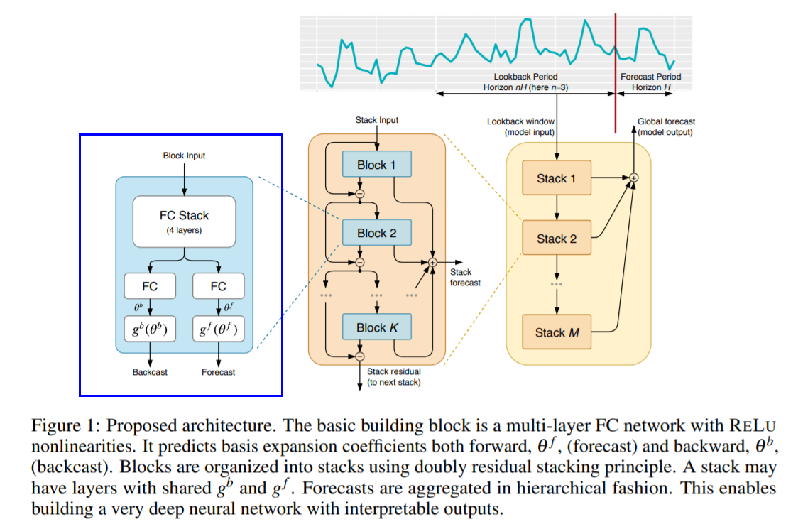
(1) Basic Block
( \(\ell\) th block에 대해 )
-
Input : \(\mathbf{x}_{\ell}\) ( = overall model input = history lookback window )
-
Output : \(\widehat{\mathbf{x}}_{\ell}\) and \(\widehat{\mathbf{y}}_{\ell}\)
Block architecture
Consists of 2 parts
**[part 1] **FC Network
- produces forward \(\theta_{\ell}^{f}\) and the backward \(\theta_{\ell}^{b}\) predictors of expansion coefficients
[part 2] backward \(g_{\ell}^{b}\) and the forward \(g_{\ell}^{f}\) basis layers
- accepts \(\theta_{\ell}^{f}\) and \(\theta_{\ell}^{b}\)
- project them on the set of basis function
- produce the “backcast \(\widehat{\mathbf{x}}_{\ell}\)” and “forecast \(\widehat{\mathbf{y}}_{\ell}\)”
Step 1)
\(\begin{aligned} \mathbf{h}_{\ell, 1} &=\mathrm{FC}_{\ell, 1}\left(\mathbf{x}_{\ell}\right), \quad \mathbf{h}_{\ell, 2}=\mathrm{FC}_{\ell, 2}\left(\mathbf{h}_{\ell, 1}\right), \quad \mathbf{h}_{\ell, 3}=\mathrm{FC}_{\ell, 3}\left(\mathbf{h}_{\ell, 2}\right), \quad \mathbf{h}_{\ell, 4}=\mathrm{FC}_{\ell, 4}\left(\mathbf{h}_{\ell, 3}\right) \\ \theta_{\ell}^{b} &=\operatorname{LINEAR}_{\ell}^{b}\left(\mathbf{h}_{\ell, 4}\right), \quad \theta_{\ell}^{f}=\operatorname{LINEAR}_{\ell}^{f}\left(\mathbf{h}_{\ell, 4}\right) \end{aligned}\).
- LINEAR : \(\theta_{\ell}^{f}=\mathbf{W}_{\ell}^{f} \mathbf{h}_{\ell, 4}\)
- FC layer : activation function of RELU
Step 2)
\(\widehat{\mathbf{x}}_{\ell}=g_{\ell}^{b}\left(\theta_{\ell}^{b}\right)\) & \(\widehat{\mathbf{y}}_{\ell}=g_{\ell}^{f}\left(\theta_{\ell}^{f}\right)\) 구하기
\[\widehat{\mathbf{y}}_{\ell}=\sum_{i=1}^{\operatorname{dim}\left(\theta_{\ell}^{f}\right)} \theta_{\ell, i}^{f} \mathbf{v}_{i}^{f}, \quad \widehat{\mathbf{x}}_{\ell}=\sum_{i=1}^{\operatorname{dim}\left(\theta_{\ell}^{b}\right)} \theta_{\ell, i}^{b} \mathbf{v}_{i}^{b}\]- \(\mathbf{v}_{i}^{f}\) and \(\mathbf{v}_{i}^{b}\) : forecast and backcast basis vectors
(2) Doubly Residual Stacking
a) Classical residual network
- adds the input of the stack of layers to its output, before passing~
b) DenseNet
- extends ResNet’s principle by introducing extra connections from the output of each stack to the input of every other stack that follows it
c) (proposed) Hierarchical Doubly Residual Stacking
problem of a) & b)
- networks structures that are DIFFICULT TO INTEPRET
- propose a novel hierarchical doubly residual topology
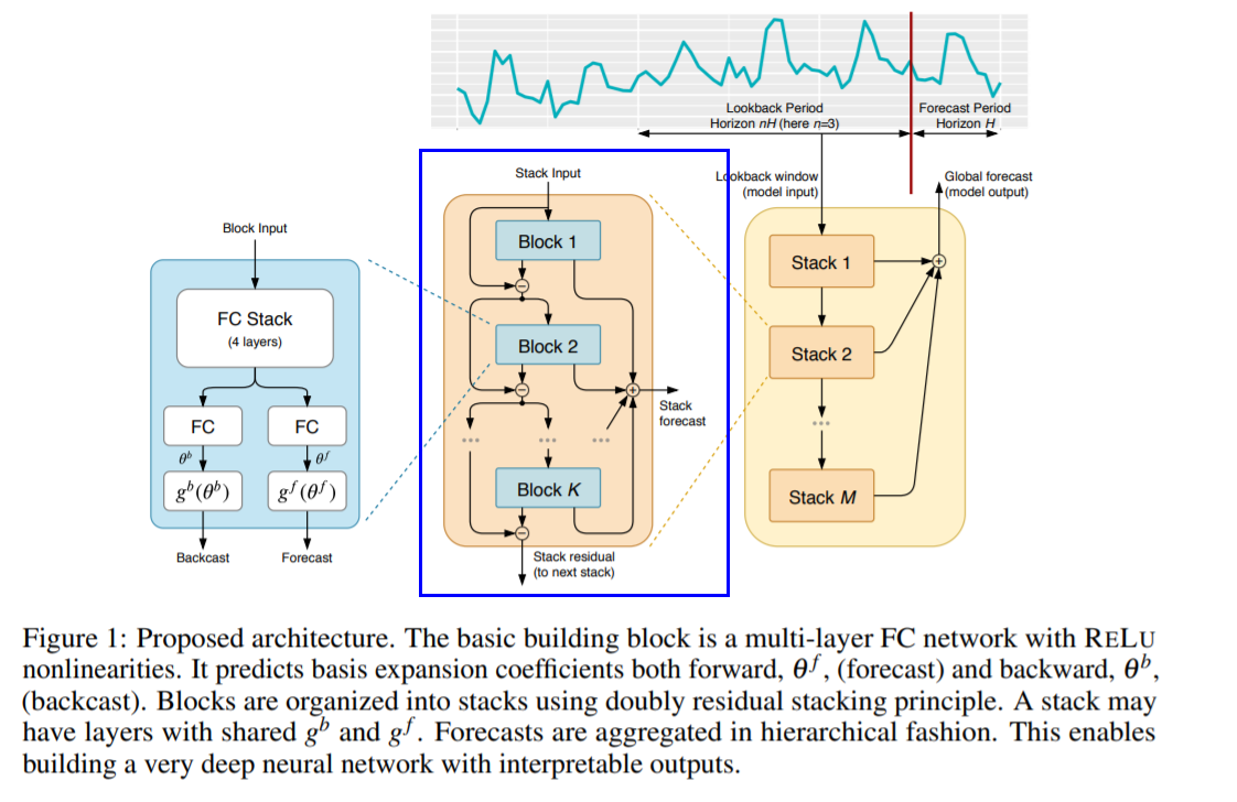
Two residual branches
- 1) running over backcast prediction of each layer
- 2) running over the forecast branch of each layer
(3) Interpretability
propose 2 configurations, based on selection of \(g_{\ell}^{b}\) and \(g_{\ell}^{f}\)
generic architecture
-
does not rely on TS-specific knowledge
-
outputs of block \(l\) :
\(\widehat{\mathbf{y}}_{\ell}=\mathbf{V}_{\ell}^{f} \boldsymbol{\theta}_{\ell}^{f}+\mathbf{b}_{\ell}^{f}, \quad \widehat{\mathbf{x}}_{\ell}=\mathbf{V}_{\ell}^{b} \boldsymbol{\theta}_{\ell}^{b}+\mathbf{b}_{\ell}^{b}\).
a) Trend model
\(\widehat{\mathbf{y}}_{s, \ell}=\sum_{i=0}^{p} \theta_{s, \ell, i}^{f} t^{i}\).
- (in matrix form) \(\widehat{\mathbf{y}}_{s, \ell}^{t r}=\mathbf{T} \theta_{s, \ell}^{f}\)
- \(\mathbf{T}=\left[\mathbf{1}, \mathbf{t}, \ldots, \mathbf{t}^{p}\right]\) : matrix of powers of \(\mathbf{t}\)
b) Seasonality model
\(\widehat{\mathbf{y}}_{s, \ell}=\sum_{i=0}^{\lfloor H / 2-1\rfloor} \theta_{s, \ell, i}^{f} \cos (2 \pi i t)+\theta_{s, \ell, i+\lfloor H / 2\rfloor}^{f} \sin (2 \pi i t)\).
- (in matrix form) \(\widehat{\mathbf{y}}_{s, \ell}^{\text {seas }}=\mathbf{S} \theta_{s, \ell}^{f}\).
- \(\mathbf{S}=[\mathbf{1}, \cos (2 \pi \mathbf{t}), \ldots \cos (2 \pi\lfloor H / 2-1\rfloor \mathbf{t})), \sin (2 \pi \mathbf{t}), \ldots, \sin (2 \pi\lfloor H / 2-1\rfloor \mathbf{t}))]\).
(4) Ensemble
more powerful regularization than dropout / L2-norm…