(paper) Time Series is a Special Sequence ; Forecasting with Sample Convolution and Interaction

Time Series is a Special Sequence ; Forecasting with Sample Convolution and Interaction (2021)

Contents

1. Abstract
2. Introduction
3. Background
   1. Quantile Regression
   2. CRPS
4. Forecasting with IQN

0. Abstract

Existing DL methods use “generic sequence models”

• ex) RNN/LSTM , Transformer ,TCN

\(\rightarrow\) ignores some unique properties of time-series!

Propose novel architecture for time-series forecast

• algorithm : SCINet

• conduct sample convolution & interaction at multiple resolutions for temporal modeling
• facilitates extracting features with enhanced predictability

1. Introduction

DL is better than traditional methods at time-series forecasting (TSF)!

3 main kinds of DNN

• 1) RNNs ( ex. LSTM & GRUs )
• 2) Transformer
• 3) TCNs ( Temporal Convolutional Networks )
  • shown to be best among three
  • combined with GNNs to solve various temporal-spatial TSF problems

TCNs

• perform “dilated causal convolutions” ( WaveNet 참고 )
• 2 principles of “dilated causal convolutions”
  • 1) network produces an output of same length as input
  • 2) no leakage from the future \(\rightarrow\) past

\(\rightarrow\) This paper argues that these 2 principles are unnecessary

SCINet ( Sample Convolution and Interaction Network )

contibutions

• 1) discover the misconception of existing TCN design principles

  ( causal convolution is NOT NECESSARY )

• 2) propose hierarchical TSF framework, SCINet

  ( based on unique attributes of time series data )

• 3) design a basic building block SCI-Block

  ( down samples input data/feature into 2 parts & extract features each )

  ( incorporate interactive learning between 2 parts )

2. Related Work & Motivation

Notation

• long time series \(\mathbf{X}^{*}\)

• look-back window of fixed length \(T\)

• forecast

  • single-step forecast : predict \(\hat{\mathbf{X}}_{t+\tau: t+\tau}=\left\{\mathbf{x}_{t+\tau}\right\}\)
  • multi-step forecast : predict \(\hat{\mathbf{X}}_{t+1: t+\tau}=\left\{\mathbf{x}_{t+1}, \ldots, \mathbf{x}_{t+\tau}\right\}\)

  based on the past \(T\) steps \(\mathbf{X}_{t-T+1: t}=\left\{\mathbf{x}_{t-T+1}, \ldots, \mathbf{x}_{t}\right\}\)

• \(\tau\) : length of the forecast horizon

• \(\mathbf{x}_{t} \in \mathbb{R}^{d}\) : value at time step \(t\) & \(d\) : number of time-series

(1) DL-based

(1) RNN-based

• internal memory ( memory state is ‘recursively’ updated )
• problem : error accumulation & gradient vanishing/exploding

(2) Transformers

• better than RNN in efficiency & effectiveness of self-attention
• quite effective in “predicting long sequence”
• problem : overhead of Transformer-based models

(3) Convolutional models

• popular choice

• parallel convolution operation of multiple filters

  \(\rightarrow\) allow for fast data processing & efficient dependencies learning

(2) Rethink Dilated Casual Convolution

Dilated Casual Convolution : first used in WaveNet

• stack of casual convolutional layers, with exponentially enlarged dilation factors

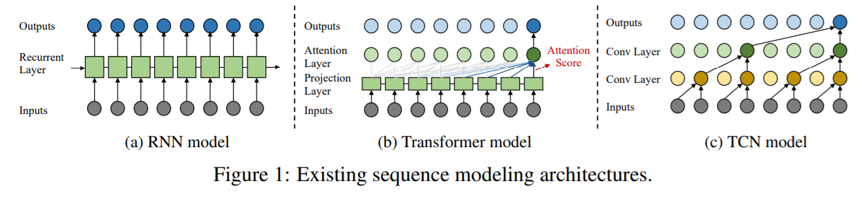
• Figure 1-(c) : Dilated Casual Convolution

TCNs are based upon 2 principles

• 1) network produces an output of same length as input
• 2) no leakage from the future \(\rightarrow\) past

\(\rightarrow\) UNNECESSARY for time series forecasting!

Principle 1) 반박

• TSF : predict some future values with a given look-back window

  따라서, 굳이 input & output length 동일할 필요 없음

Principle 2) 반박

• causality가 필요하긴 하지만, 그러한 information leakage problem은 output과 input이 temporal overlap을 가질때만!
• 미래의 known 정보일 경우 굳이 차단할 필요 없음!

3. SCINet : Sample Convolution and Interaction Networks

hierarchical framework that enhances predictability of the original time series,

by capturing temporal dependencies at multiple temporal resolutions

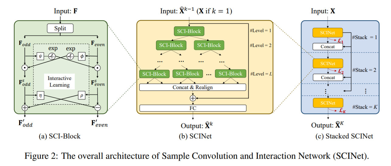
(1) SCI-Block

basic building block of SCINet

Steps

• Step 1) [Splitting] downsamples input into 2 sub-sequences
• Step 2) process each sub-sequence with distinct conv filter
• Step 3) [Interactive-learning] incorporate interactive learning between 2 sub-sequences

Notation

• \(\mathbf{F}_{\text {odd }}^{s}=\mathbf{F}_{\text {odd }} \odot \exp \left(\phi\left(\mathbf{F}_{\text {even }}\right)\right)\).
• \(\mathbf{F}_{\text {even }}^{s}=\mathbf{F}_{\text {even }} \odot \exp \left(\psi\left(\mathbf{F}_{o d d}\right)\right)\).
• \(\mathbf{F}_{o d d}^{\prime}=\mathbf{F}_{\text {odd }}^{s} \pm \rho\left(\mathbf{F}_{\text {even}}^{s}\right)\).
• \(\mathbf{F}_{\text {even }}^{\prime}=\mathbf{F}_{\text {even }}^{s} \mp \eta\left(\mathbf{F}_{o d d}^{s}\right)\).

(2) SCI-Net

• binary tree structure

• realign & concatenate all the low-resolution components into new sequence representation

  & add it to the original series

(3) Stacked SCINet with Intermediate Supervision

• to fully accumulate the historical info within the look-back window, further stack \(K\) SCI-Nets

• apply intermediate supervision

  \(\rightarrow\) to ease the learning of intermediate temporal features

(4) Loss Function

Loss of the \(k\)-th intermediate prediction

• \(\mathcal{L}_{k}=\frac{1}{\tau} \sum_{i=0}^{\tau} \mid \mid \hat{\mathbf{x}}_{i}^{k}-\mathbf{x}_{i} \mid \mid , \quad k \neq K\).

Loss of final SCINet

• (multi-step) same as above
• (single-step) \(\mathcal{L}_{K}=\frac{1}{\tau-1} \sum_{i=0}^{\tau-1} \mid \mid \hat{\mathbf{x}}_{i}^{K}-\mathbf{x}_{i} \mid \mid +\lambda \mid \mid \hat{\mathbf{x}}_{\tau}^{K}-\mathbf{x}_{\tau} \mid \mid\)
  • \(\lambda \in (0,1)\) : balancing parameter

Total Loss : \(\mathcal{L}=\sum_{k=1}^{K} \mathcal{L}_{k}\)