
SOM-VAE : Interpretable Discrete Representation Learning on Time Series (2019)
Contents
- Abstract
- Introduction
- Probabilistic SOM-VAE
- Introducing Topological Structure in the latent space
- Encouraging Smoothness over Time
0. Abstract
HIGH-DIM time series is common!
-
could benefit from interpretable LOW-DIM representations
( but most algorithms for t.s are difficult to interpret )
Propose a new representation learning framework
-
allows to learn DISCRETE representation
\(\rightarrow\) smooth & interpretable embeddings with superior clustering performance
-
non-differentiability in discrete representation?
\(\rightarrow\) introduce gradient-based version of SOM
-
allow for probabilistic interpretation of our method, by using Markov model in latent space
1. Introduction
Interpretable representation learning = uncovering the latent structure
Many unsupervised methods ….. neglect “temporal structure” & “smooth behaviour over time”
\(\rightarrow\) need clustering, where cluster assume a topological structure in low-dim sppace
( such that representations of t.s retain their smoothness in that space )
Define “Temporal Smoothness” in discrete representation space
- “topological neighborhood relationship”
- ex) SOM
- map states from uninterpretable continuous space to low-dim space, with pre-defined topolgically interpretable structure
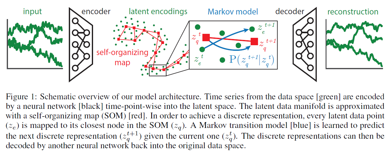
Propose a novel deep arcthitecture,
1) that learns ”topologically interpretable discrete representations” in a probabilistic fashion
2) develop a ”gradient-based version of SOM”
2. Probabilistic SOM-VAE
2-1. Introducing Topological Structure in the latent space
Notation
- input : \(x \in \mathbb{R}^{d}\)
- latent encoding 1 : \(z_{e} \in \mathbb{R}^{m}\) ……….. \(z_{e}=f_{\theta}(x)\)
- latent encoding 2 : \(z_{q} \in \mathbb{R}^{m}\) ……….. dictionary \(E=\left\{e_{1}, \ldots, e_{k} \mid e_{i} \in \mathbb{R}^{m}\right\}\) by \(z_{q} \sim p\left(z_{q} \mid z_{e}\right)\).
- categorical : \(p\left(z_{q} \mid z_{e}\right)=\mathbb{1}\left[z_{q}=\arg \min _{e \in E}\left \mid \mid z_{e}-e\right \mid \mid ^{2}\right]\).
- reconstruction of input : \(\hat{x}\) . ………..\(\widehat{x}=g_{\phi}(z)\)
- \(\hat{x}_{e}=g_{\phi}\left(z_{e}\right)\) .
- \(\hat{x}_{q}=g_{\phi}\left(z_{q}\right)\).
- \(k\) nodes of SOM : \(V=\left\{v_{1}, \ldots, v_{k}\right\}\), where every node corresponds to….
- embedding in the data space \(e_{v} \in \mathbb{R}^{d}\)
- representation in a lower-dimensional discrete space \(m_{v} \in M\)
- training data : \(\mathcal{D}=\left\{x_{1}, \ldots, x_{n}\right\}\)
training procedure : ( use 2D SOM )
- winner node \(\tilde{v}\) is chosen for every point \(x_{i}\)
- according to \(\tilde{v}=\arg \min _{v \in V}\left \mid \mid e_{v}-x_{i}\right \mid \mid ^{2}\)
- embedding vector for every node \(u \in V\) is then updated
- according to \(e_{u} \leftarrow e_{u}+N\left(m_{u}, m_{\tilde{v}}\right) \eta\left(x_{i}-e_{u}\right)\),
- \(N\left(m_{u}, m_{\tilde{v}}\right)\) : neighborhood function
end-to-end
-
cannot use the standard SOM training algorithm
-
devise a loss function term whose gradient corresponds to a weighted version of the original SOM update
-
any time an embedding \(e_{i, j}\) at position \((i, j)\) in the map gets updated,
also updates all the embeddings in its immediate neighborhood \(N\left(e_{i, j}\right)\).
-
neighborhood : \(N\left(e_{i, j}\right)=\left\{e_{i-1, j}, e_{i+1, j}, e_{i, j-1}, e_{i, j+1}\right\}\)
-
loss function for a single \(x\) :
- \(\mathcal{L}_{\text {SOM-VAE }}\left(x, \hat{x}_{q}, \hat{x}_{e}\right)=\mathcal{L}_{\text {reconstruction }}\left(x, \hat{x}_{q}, \hat{x}_{e}\right)+\alpha \mathcal{L}_{\text {commitment }}(x)+\beta \mathcal{L}_{\text {SOM }}(x)\).
-
term 1) \(\mathcal{L}_{\text {reconstruction }}\left(x, \hat{x}_{q}, \hat{x}_{e}\right)=\left \mid \mid x-\hat{x}_{q}\right \mid \mid ^{2}+\left \mid \mid x-\hat{x}_{e}\right \mid \mid ^{2}\)
-
first term : discrete reconstruction loss
-
corresponds to the ELBO of the VAE
( assume a uniform prior over \(z_{q}\), the KL-term in the ELBO is constant …ignored )
-
-
term 2) \(\mathcal{L}_{\text {commitment }}(x)=\left \mid \mid z_{e}(x)-z_{q}(x)\right \mid \mid ^{2}\)
- due to the nondifferentiability of the embedding assignment, \(\mathcal{L}_{\text {commitment }}\) term has to be explicitly added
-
term 3) \(\mathcal{L}_{\text {SOM }}(x)=\sum_{\tilde{e} \in N\left(z_{q}(x)\right)}\left \mid \mid \tilde{e}-\operatorname{sg}\left[z_{e}(x)\right]\right \mid \mid ^{2}\)
- \(\mathrm{sg}[\cdot]\) : gradient stopping operator
-
2-2. Encouraging Smoothness over Time
ultimate goal : predict the development of t.s in interpretable way
1) should be interpreteable 2) should predict well
\(\rightarrow\) Use temporal probabilistic model
Exploit low-dim discrete space induced by SOM to learn a temporal model
model is learned joinlty with SOM-VAE
Loss Function
\(\mathcal{L}\left(x^{t-1}, x^{t}, \hat{x}_{q}^{t}, \hat{x}_{e}^{t}\right)=\mathcal{L}_{\text {SOM-VAE }}\left(x^{t}, \hat{x}_{q}^{t}, \hat{x}_{e}^{t}\right)+\gamma \mathcal{L}_{\text {transitions }}\left(x^{t-1}, x^{t}\right)+\tau \mathcal{L}_{\text {smoothness }}\left(x^{t-1}, x^{t}\right)\).
-
term 1) cluster
-
term 2) prediction
-
\(\mathcal{L}_{\text {transitions }}\left(x^{t-1}, x^{t}\right)=-\log P_{M}\left(z_{q}\left(x^{t-1}\right) \rightarrow z_{q}\left(x^{t}\right)\right)\),
( \(P_{M}\left(z_{q}\left(x^{t-1}\right) \rightarrow z_{q}\left(x^{t}\right)\right)\) : probability of a transition from state \(z_{q}\left(x^{t-1}\right)\) to state \(z_{q}\left(x^{t}\right)\) in the Markov model. )
-
-
term 3) smoothing
- \(\mathcal{L}_{\text {smoothness }}\left(x^{t-1}, x^{t}\right)=\mathbb{E}_{P_{M}\left(z_{q}\left(x^{t-1}\right) \rightarrow \tilde{e}\right)}\left[\left \mid \mid \tilde{e}-z_{e}\left(x^{t}\right)\right \mid \mid ^{2}\right]\).