(paper)Temporal Latent Auto-Encoder ; A Method for Probabilistic Multivariate Time Series Forecasting

Temporal Latent Auto-Encoder ; A Method for Probabilistic Multivariate Time Series Forecasting (2021)

Contents

1. Abstract

2. Introduction

3. Problem Setup & Methodology

   1. Point Prediction
   2. Probabilistic Prediction

0. Abstract

Probabilistic Forecasting of high-dim MTS : 어렵다!

기존 연구 방향

• 1) simple distribution assumption
• 2) cross-series correlation 고려 X

Propose a novel “temporal latent auto-encoder”

• “non-linear” factorization of MTS
• end-to-end

1. Introduction

Forecasting in multivariate settings

• 방법 1) 모든 time-series를 예측하는 1개의 multi-output model

• 방법 2) 모든 time-series를 각각의 모델로 fitting 시키기 ( separate model )

  \(\rightarrow\) 문제점 : unable to model “cross-series” correlation

• 해결책 : factorization 사용하자!

  • relationships between time series are factorized into a low rank matrix

  ( each time series = linear combination of a smaller set of latent/basis time series )

DeepGLO

• enable non-linear latent space forecast models
• iteratively alternates between
  • 1) linear matrix factorization
  • 2) fitting a latent space TCN (Temporal CNN)
• forecasts from this model are then fed as covariates to a separately trained multi-task univariate TCN model

Key Limitations of DeepGLO

1. series 사이의 non-linear relationship는 포착 불가
2. end-to-end가 아님
3. probabilistic output이 아님
4. limited to capture “stationary” relationships between time series

TLAE (Temporal Latent Autoencoder)

• enbales “non-linear” transforms of input series
• end-to-end
• infers joint predictive distribution

2. Problem Setup & Methodology

Notation

• multivariate ts : bold CAPITAL letter
• univariate ts : bold LOWERCASE letter
• ts data : \(\mathbf{X}\)
  • \(\mathbf{x}_{i}\) : \(i\) -th column
  • \(x_{i, j}\) : \((i, j)\)-th entry of \(\mathbf{X}\)
  • \(\mid \mid \mathbf{X} \mid \mid _{\ell_{2}}\) : matrix Frobenius norm
  • \(\mid \mid \mathrm{x} \mid \mid _{\ell_{p}}\) : \(\ell_{p}\) -norm of the vector \(\mathrm{x}\) ( = \(\left(\sum_{i} x_{i}^{p}\right)^{1 / p}\) )
• \[\mathbf{Y} \in \mathbb{R}^{n \times T}\]
  • \(\mathbf{Y}_{B}\) : sub-matrix of \(\mathrm{Y}\) with column indices in \(B\).
  • \(\mid \mathcal{B} \mid\) : cardinality of this set

Problem definition

• collection of high-dim multivariate time series : \(\left(\mathbf{y}_{1}, \ldots, \mathbf{y}_{T}\right)\)

• problem of forecasting \(\tau\) future values : \(\left(\mathbf{y}_{T+1}, \ldots, \mathbf{y}_{T+\tau}\right)\)

  ( given \(\left\{\mathbf{y}_{i}\right\}_{i=1}^{T}\) )

• decomposition : \(p\left(\mathbf{y}_{T+1}, \ldots, \mathbf{y}_{T+\tau} \mid \mathbf{y}_{1: T}\right)=\prod_{i=1}^{\tau} p\left(\mathbf{y}_{T+i} \mid \mathbf{y}_{1: T+i-1}\right)\) 풀기

(1) Point Prediction

Motivation

• TRMF (Temporal Regularized Matrix Factorization) : decomposes MTS ( = \(\mathbf{Y} \in \mathbb{R}^{n \times T}\) ) with
  • (1) \(\mathbf{F} \in \mathbb{R}^{n \times d}\)
  • (2) \(\mathbf{X} \in \mathbb{R}^{d \times T}\)………. imposing temporal constraints
• 만약 \(\mathbf{Y}\)가 few time series in \(\mathbf{X}\)로 잘 대변된다면, 더 low-dimension으로도 축소 가능!

RNN과 같은 (temporal DNN) 모델들을 학습시키기 위해, data는 temporally하게 batch로 나눠진다.

• \(\mathbf{Y}_{B}\) : a batch of data containing a subset of \(b\) time samples

  ( \(\mathbf{Y}_{B}=\left[\mathbf{y}_{t}, \mathbf{y}_{t+1}, \ldots, \mathbf{y}_{t+b-1}\right]\) where \(B=\) \(\{t, \ldots, t+b-1\}\) are time indices )

constrained factorization 풀기

• \(\min _{\mathbf{X}, \mathbf{F}, \mathbf{W}} \mathcal{L}(\mathbf{X}, \mathbf{F}, \mathbf{W})=\frac{1}{ \mid \mathcal{B} \mid } \sum_{B \in \mathcal{B}} \mathcal{L}_{B}\left(\mathbf{X}_{B}, \mathbf{F}, \mathbf{W}\right)\).

  where \(\mathcal{B}\) is the set of all data batches

• each batch loss :

  \(\mathcal{L}_{B}\left(\mathbf{X}_{B}, \mathbf{F}, \mathbf{W}\right) \triangleq \frac{1}{n b} \mid \mid \mathbf{Y}_{B}-\mathbf{F} \mathbf{X}_{B} \mid \mid _{\ell_{2}}^{2}+\lambda \mathcal{R}\left(\mathbf{X}_{B} ; \mathbf{W}\right)\).

  • \(\mathcal{R}\left(\mathbf{X}_{B} ; \mathbf{W}\right)\) : regularization parameterized

• temporal constraint 위해… autoregressive model on \(\mathbf{X}_{B}\)

  • \(\mathbf{x}_{\ell}=\sum_{j=1}^{L} \mathbf{W}^{(j)} \mathbf{x}_{\ell-j}\). ( \(L\) : predefined lag parameter )

• Regularization :

  • (기본) \(\mathcal{R}\left(\mathbf{X}_{B} ; \mathbf{W}\right) \triangleq \sum_{\ell=L+1}^{b} \mid \mid \mathbf{x}_{\ell}-\sum_{j=1}^{L} \mathbf{W}^{(j)} \mathbf{x}_{\ell-j} \mid \mid _{\ell_{2}}^{2}\).
  • (TCN) \(\mathcal{R}\left(\mathbf{X}_{B} ; \mathbf{W}\right) \triangleq \sum_{\ell=L+1}^{b} \mid \mid \mathbf{x}_{\ell}-\operatorname{TCN}\left(\mathbf{x}_{\ell-L, \ldots, \mathbf{x}_{\ell-1}} ; \mathbf{W}\right) \mid \mid _{\ell_{2}}^{2}\)

Our Model

if \(\mathrm{Y}\) can be decomposed by \(\mathbf{F}\) and \(\mathbf{X}\)…

• \(\mathbf{X}=\mathbf{F}^{+} \mathbf{Y}\) where \(\mathbf{F}^{+}\) is the pseudo-inverse of \(\mathbf{F}\)
• \(\mathbf{Y}=\mathbf{F F}^{+} \mathbf{Y}\).

if \(\mathbf{F}^{+}\) can be replaced by an encoder and \(\mathbf{F}\) by a decoder…

\(\rightarrow\) exploit the ideas of AE

• Latent representation : \(\mathbf{X}=g_{\phi}(\mathbf{Y})\)
• reconstruction of \(\mathbf{Y}\) : \(\hat{\mathbf{Y}}=f_{\boldsymbol{\theta}}(\mathbf{X})\)

LSTM network

• enc & dec 사이에 temporal structure of the latent representation를 잡을 수 있는 layer를 넣음

• encode long-range dependency of latent variables

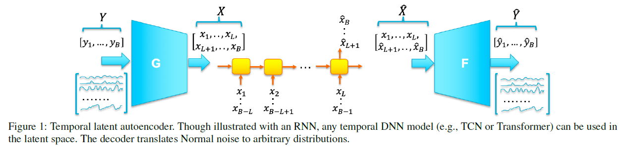
Flow

• 1) a batch of the time series \(\mathbf{Y}_{B}=\left[\mathbf{y}_{1}, \ldots, \mathbf{y}_{b}\right] \in \mathbb{R}^{n \times b}\) is

  ​ embedded into the latent variables \(\mathbf{X}_{B}=\left[\mathbf{x}_{1}, \ldots, \mathbf{x}_{b}\right] \in \mathbb{R}^{d \times b}\)

• 2) These sequential ordered \(\mathrm{x}_{i}\) are input to the LSTM to produce outputs \(\hat{\mathbf{x}}_{L+1}, \ldots, \hat{\mathbf{x}}_{b}\)

  ​ with each \(\hat{\mathbf{x}}_{i+1}= h_{\mathrm{W}}\left(\mathrm{x}_{i-L+1}, \ldots, \mathrm{x}_{i}\right)\)

• 3) decoder will take the matrix \(\hat{\mathbf{X}}_{B}\) consisting of variables \(\mathrm{x}_{1}, \ldots, \mathrm{x}_{L}\) and \(\hat{\mathrm{x}}_{L+1}, \ldots, \hat{\mathrm{x}}_{b}\) as input

  ​ and yield \(\hat{\mathbf{Y}}_{B}\)

batch output \(\hat{Y}_{B}\) contains two components

• 1) \(\hat{\mathbf{y}}_{i}\) with \(i=1, \ldots, L\)
  • directly transferred from the encoder without passing through the middle layer
  • \(\hat{\mathbf{y}}_{i}=f_{\boldsymbol{\theta}} \circ g_{\boldsymbol{\phi}}\left(\mathbf{y}_{i}\right)\).
• 2) \(\hat{\mathbf{y}}_{i}\) with \(i=L+1, \ldots, b\)
  • function of the past input
  • \(\hat{\mathbf{y}}_{i+1}=f_{\boldsymbol{\theta}} \circ h_{\mathbf{W}} \circ g_{\boldsymbol{\phi}}\left(\mathbf{y}_{i-L+1}, \ldots, \mathbf{y}_{i}\right)\).
• minimize \(\mid \mid \hat{\mathbf{y}}_{i}-\mathbf{y}_{i} \mid \mid _{\ell_{p}}^{p}\)

Objective function w.r.t batch of data :

• \(\mathcal{L}_{B}(\mathbf{W}, \boldsymbol{\phi}, \boldsymbol{\theta}) \triangleq \frac{1}{n b} \mid \mid \mathbf{Y}_{B}-\hat{\mathbf{Y}}_{B} \mid \mid _{\ell_{p}}^{p} +\lambda \frac{1}{d(b-L)} \sum_{i=L}^{b-1} \mid \mid \mathbf{x}_{i+1}-h_{\mathbf{W}}\left(\mathbf{x}_{i-L+1}, \ldots, \mathbf{x}_{i}\right) \mid \mid _{\ell_{q}}^{q}\).

Overall Loss Function :

• \(\min _{\mathbf{W}, \phi, \theta} \mathcal{L}(\mathbf{W}, \phi, \boldsymbol{\theta})=\frac{1}{ \mid \mathcal{B} \mid } \sum_{B \in \mathcal{B}} \mathcal{L}_{B}(\mathbf{W}, \phi, \boldsymbol{\theta})\).

Interpretation

• \(\mathbf{Y}\) & \(\hat{\mathbf{Y}}\) 가깝도록 :

  capture the correlation cross time series and encode this global info into few latent variables \(\mathbf{X}\)

• \(\hat{\mathbf{X}}\) & \(\mathbf{X}\) 가깝도록 :

capture temporal dependency and provide the predictive capability of the latent representation

(2) Probabilistic prediction

input space를 direct하게 모델링하지 않고,

encode high-dim data to low-dim embedding

\(\rightarrow\) 이 과정에서 probabilistic model을 사용

\[p\left(\mathbf{x}_{i+1} \mid \mathbf{x}_{1}, \ldots, \mathbf{x}_{i}\right)=\mathcal{N}\left(\mathbf{x}_{i+1} ; \boldsymbol{\mu}_{i}, \boldsymbol{\sigma}_{i}^{2}\right), \quad i=L, \ldots, b\]

• \(\boldsymbol{\mu}_{i}=h_{\mathbf{W}}^{(1)}\left(\mathbf{x}_{1}, \ldots, \mathbf{x}_{i}\right)\) and \(\boldsymbol{\sigma}_{i}^{2}=h_{\mathbf{W}}^{(2)}\left(\mathbf{x}_{1}, \ldots, \mathbf{x}_{i}\right)\)

Objective function \(\mathcal{L}_{B}(\phi, \theta, \mathbf{W})\)

• weighted combination of the reconstruction loss and the negative log likelihood loss

• \(\frac{1}{n b} \mid \mid \hat{\mathbf{Y}}_{B}-\mathbf{Y}_{B} \mid \mid _{\ell_{p}}^{p}-\lambda \frac{1}{b-L} \sum_{i=L+1}^{b} \log \mathcal{N}\left(\mathbf{x}_{i} ; \boldsymbol{\mu}_{i-1}, \boldsymbol{\sigma}_{i-1}^{2}\right)\).

• VAE와 유사한 꼴

  • 1) data reconstruction loss
  • 2) KL-divergence loss ( encourage latent distn to be close to standard Gaussian )

• VAE와의 차이점 :

  our model has a temporal model in the “latent space” & measure a “conditional discrepancy”