(paper) A Transformer-based Framework for Multivariate Time Series Representation Learning

A Transformer-based Framework for Multivariate Time Series Representation Learning (2020)

Contents

1. Abstract
2. Introduction
3. Related Works
   1. Regression & Classification of ts
   2. Unsupervised learning for mts
   3. Transformer for ts
4. Methodology
   1. Base model
   2. Regression & Classification
   3. Unsupervised pre-training

0. Abstract

propose “Transformer-based” framework for “unsupervised representation learning” of MTS

Pre-trained models, for downstream task

• forecasting, missing value imputation

1. Introduction

• MTS 데이터는 넘쳐나지만, labeled data는 충분하지 않다!

• NLP/CV에 비해, TS를 위한 DL은 아직…

• Transformer 핵심 : “multi-head attention”

• 제안한 알고리즘

  • 1) transformer 사용해서 dense vector representation을 뽑아내!

    ( through input denoising objective )

  • 2) 그렇게 학습한 pre-trained model을 여러 downstream task에 적용

    ( regression ,classification, imputation, forecasting )

2. Related Works

(1) Regression & Classification of ts

Non-DL

• TS-CHIEF (2020) & HIVE-COTE(2018)
  • very sophisticated methods
  • heterogeneous ensembles of classifiers
• ROCKET(2020) :
  • fast method
  • train linear classifier on top of features, extracted by a flat collection of numerous & various random convolutional kernels

DL ( CNN-based )

• InceptionTime(2019)
• ResNet (2019)

(2) Unsupervised learning for mts

• usually employ “autoencoders”

(3) Transformer for ts

1. Li et al (2019)
   • univariate time series forecasting
2. Wu et al (2020)
   • forecast influenza prevalence
3. Ma et al (2019)
   • variant of self-attention for imputation of missing values in multivariate, geo-tagged ts
4. This paper
   • generalize the use of transformers from solutions to specific generative tasks
   • wide variety of downstream tasks ( like BERT )

3. Methodology

(1) Base Model

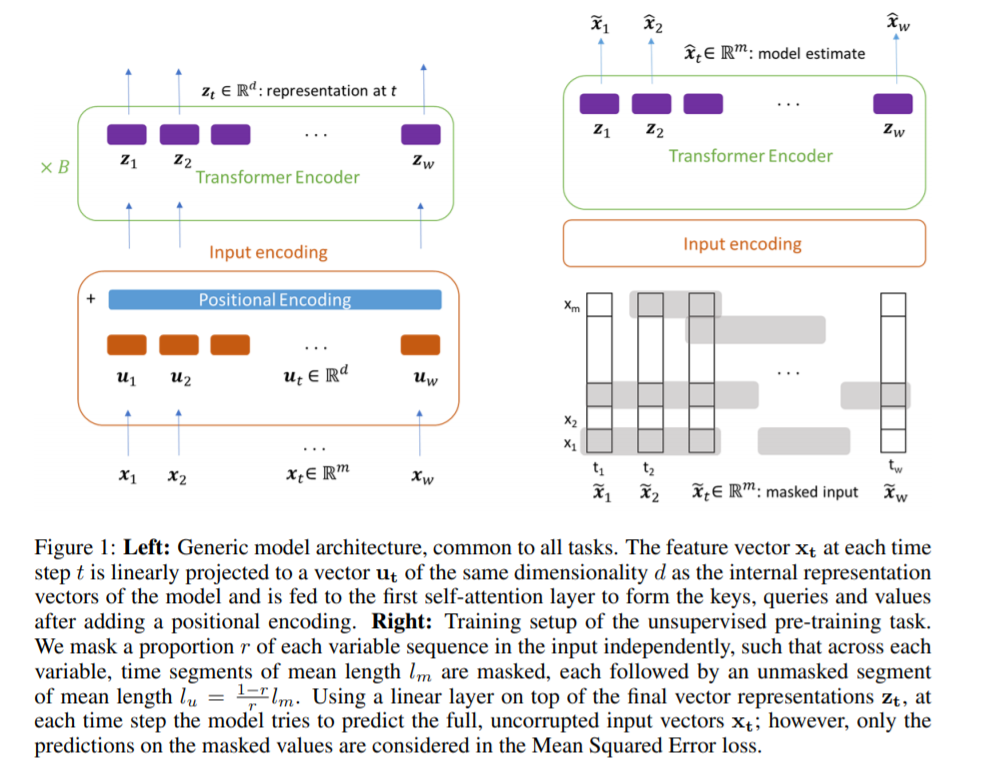
transformer ENCODER (O), DECODER (X)

Notation

• training samples : \(\mathbf{X} \in \mathbb{R}^{w \times m}\)
  • length : \(w\)
  • number of variables : \(m\)
  • \(\mathbf{x}_{\mathbf{t}} \in \mathbb{R}^{m}\).
• \(\mathbf{X} \in \mathbb{R}^{w \times m}=\left[\mathrm{x}_{1}, \mathrm{x}_{2}, \ldots, \mathrm{x}_{\mathrm{w}}\right]\).

Basic steps

Step 1) \(\mathrm{x}_{\mathbf{t}}\) are first normalized

Step 2) then linearly projected onto a \(d\) dimension

• \(\mathbf{u}_{\mathbf{t}}=\mathbf{W}_{\mathbf{p}} \mathbf{x}_{\mathbf{t}}+\mathbf{b}_{\mathbf{p}}\)…… where \(\mathbf{W}_{\mathbf{p}} \in \mathbb{R}^{d \times m}, \mathbf{b}_{\mathbf{p}} \in \mathbb{R}^{d}\).

• will become the queries, keys and values of the self-attention layer, after adding the positional encodings and multiplying by the corresponding matrices.

Optional

• \(\mathbf{u}_{\mathbf{t}}\) need not necessarily be obtained from the (transformed) feature vectors at a time step \(t\) :

• instead, use a 1D-convolutional layer with 1 input and \(d\) output channels and kernels \(K_{i}\) of size \((k, m)\), where \(k\) is the width in number of time steps and \(i\) the output channel

  \(u_{t}^{i}=u(t, i)=\sum_{j} \sum_{h} x(t+j, h) K_{i}(j, h), \quad i=1, \ldots, d\).

Step 3) add positional encodings

• \(W_{\text {pos }} \in \mathbb{R}^{w \times d}\).
• \(U \in \mathbb{R}^{w \times d}=\left[\mathbf{u}_{1}, \ldots, \mathbf{u}_{\mathbf{w}}\right]\).

• \(U^{\prime}=U+W_{\text {pos }}\).

• use fully learnable positional encodings

Step 4) Batch Normalization

• mitigate effect of outlier values in time series

  ( not an issue in NLP )

(2) Regression & Classification

final representation vectors \(\mathbf{z}_{\mathbf{t}} \in \mathbb{R}^{d}\).

\(\rightarrow\) all time steps are concatenated into a single vector \(\overline{\mathbf{z}} \in \mathbb{R}^{d \cdot w}=\) \(\left[\mathbf{z}_{1} ; \ldots ; \mathbf{z}_{\mathbf{w}}\right]\)

becomes an input to a linear output layer with parameters \(\mathbf{W}_{\mathbf{o}} \in \mathbb{R}^{n \times(d \cdot w)}\),

• \(\hat{\mathbf{y}}=\mathbf{W}_{\mathbf{o}} \overline{\mathbf{z}}+\mathbf{b}_{\mathbf{o}}\).
• \(n\) :
  • number of scalars to be estimated for the regression problem (typically \(n=1\) )
  • number of classes for the classification problem

loss of single data ( in regression )

• \(\mathcal{L}= \mid \mid \hat{\mathbf{y}}-\mathbf{y} \mid \mid ^{2}\).

(3) Unsupervised pre-training

“AUTOREGRESSIVE task of denoising the input”

• part of input to 0 & ask to predict the masked value!
• binary noise mask \(\mathbf{M} \in \mathbb{R}^{w \times m}\)
• input is masked by element-wise multiplication : \(\tilde{\mathbf{X}}=\mathbf{M} \odot \mathbf{X}\)
• proportion \(r\) of each mask column is set oto 0

Loss

• output : \(\hat{\mathbf{x}}_{\mathbf{t}}\)of the full, uncorrupted input vectors \(\mathrm{x}_{\mathrm{t}}\)
  • \(\hat{\mathbf{x}}_{\mathbf{t}}=\mathbf{W}_{\mathbf{o}} \mathbf{z}_{\mathbf{t}}+\mathbf{b}_{\mathbf{o}}\).
• however, only the predictions on the masked values are considered in MSE
  • \(\mathcal{L}_{\mathrm{MSE}}=\frac{1}{ \mid M \mid } \sum_{(t, i) \in M}(\hat{x}(t, i)-x(t, i))^{2}\).