TimesURL; Self-supervised Contrastive Learning for Universal Time Series Representation Learning

TimesURL: Self-supervised Contrastive Learning for Universal Time Series Representation Learning

Contents

1. Abstract
2. Problem Formulation
3. Method Introduction
4. FTAug Method
   1. Frequency Mixing
   2. Random Cropping
5. Double Universum Learning
6. CL for Segment-level Information
7. Time Reconstruction for Instance-level Information

Abstract

Learning universal TS representations

• Self-supervised contrastive learning (SSCL)

Due to the special temporal characteristics, hard for TS domain!

Three parts involved in SSCL

• (1) Designing augmentation methods for positive pairs
• (2) Constructing (hard) negative pairs
• (3) Designing SSCL loss

(1) & (2)

• Unsuitable positive and negative pair construction may introduce inappropriate inductive biases

(3)

• Just exploring segment- or instance-level semantics information is not enough

TimesURL

Propose a novel SSL framework

Three proposals

• a) Introduce a frequency-temporal-based augmentation
  • to keep the temporal property unchanged
• b) Construct double Universums as a special kind of hard negative
• c) Introduce time reconstruction as a joint optimization objective along with CL
  • to capture both segment-level and instance-level information

Various tasks

• Short- and long-term forecasting
• Imputation
• Classification
• Anomaly detection
• Transfer learning

1. Problem Formulation

• Nonlinear embedding function \(f_\theta\),

• TS set \(\mathcal{X}=\left\{x_1, x_2, \ldots, x_N\right\}\)
  • Each input TS: \(x_i \in \mathbb{R}^{T \times F}\),
• Representation \(r_i=\left\{r_{i, 1}, r_{i, 2}, \ldots, r_{i, T}\right\}\),
  • \(r_{i, t} \in \mathbb{R}^K\) is the representation vector at time \(t\),

2. Method Introduction

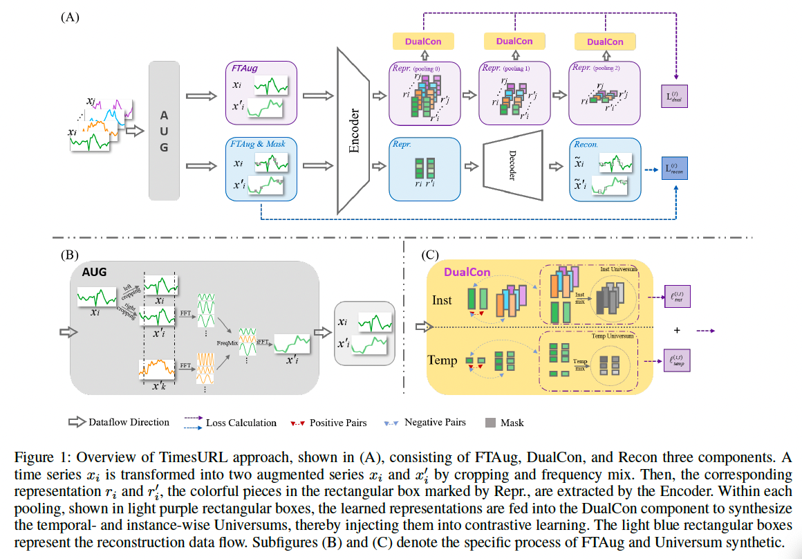
Step 1) Generate augmentation sets \(\mathcal{X}^{\prime}\) and \(\mathcal{X}_M^{\prime}\)

• through FTAug
• for original series \(\mathcal{X}\) and masked series \(\mathcal{X}_M\)

Step 2) Get two pairs of original and augmentation series sets

• (1) \(\left(\mathcal{X}, \mathcal{X}^{\prime}\right)\) for contrastive learning
• (2) \(\left(\mathcal{X}_M, \mathcal{X}_M^{\prime}\right)\) for time reconstruction

Step 3) Map the above sets with \(f_\theta\)

Encourage \(\mathcal{R}\) and \(\mathcal{R}^{\prime}\) to have transformation consistency

Design a reconstruction method to precisely recover the original dataset \(\mathcal{X}\) using both \(\mathcal{R}_M\) and \(\mathcal{R}_M^{\prime}\).

Effectiveness of the model: by …

• (1) Using a suitable augmentation method for positive pair construction
• (2) Having a certain amount of hard negative samples for model generalization
• (3) Optimizing the encoder \(f_\theta\) by
  • a) CL loss
  • b) Time reconstruction loss

3. FTAug Method

Contextual consistency strategy (Yue et al. 2022)

• Same timestamp in two augmented contexts = Positive pairs

FTAug

• Combines the advantages in both (1) frequency and (2) temporal domains
• Generate the augmented contexts by ..
  • (1) Frequency mixing
  • (2) Random cropping

(1) Frequency mixing

To produce a new context view by replacing a certain rate of the frequency components

• Fast Fourier Transform (FFT)
  • with the same frequency components of another \(x_k\) in the same batc
• Inverse FFT
  • to convert back to get

Exchanging frequency components between samples

• Do not introduce unexpected noise or artificial periodicities
• Offer more reliable augmentations

(2) Random cropping

Randomly sample two overlapping time segments: \(\left[a_1, b_1\right]\), \(\left[a_2, b_2\right]\)

CL & Time reconstruction

• Optimize the representation in the overlapping segment \(\left[a_2, b_1\right]\).

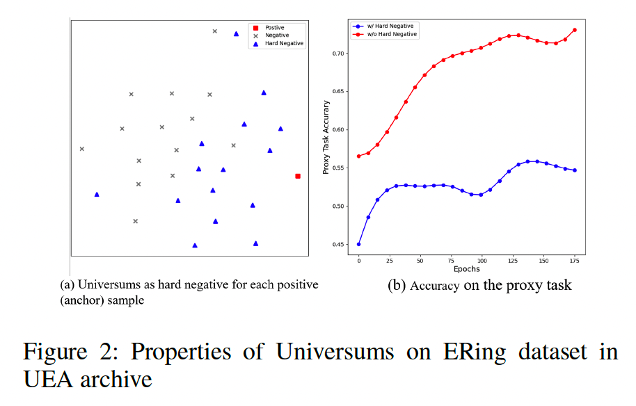
4. Double Universum Learning

Hard negative samples

• Play an important role in CL
• Have never been explored in the TS domain.
• Due to the local smoothness and the Markov property in TS…
  • Most negative samples are “easy” negative samples
  • ex) ERing dataset in UEA archive (Figure 2)

Double Universums

• Mixup Induced Universums (Han and Chen 2023; Vapnik 2006; Chapelle et al. 2007)
  • in both instance- and temporal-wise
  • Anchor-specific mixing in the embedding space
    • Mixes the specific positive feature (anchor) with the negative features for unannotated datasets.
• (1) Temporal-wise Universums
• (2) Instance-wise Universums

(1) Temporal-wise Universums

( for the \(i\)-th TS at timestamp \(t\) )

• \(\begin{aligned} & r_{i, t}^{\text {temp }}=\lambda_1 \cdot r_{i, t}+\left(1-\lambda_1\right) \cdot r_{i, t^{\prime}}, \\ & r_{i, t}^{\prime \text {temp }}=\lambda_1 \cdot r_{i, t}^{\prime}+\left(1-\lambda_1\right) \cdot r_{i, t^{\prime}}^{\prime}, \end{aligned}\).
  • \(t^{\prime}\) : Randomly chosen from \(\Omega\), the set of timestamps within the overlap of the two subseries, and \(t^{\prime} \neq t\).

(2) Instance-wise Universums

( indexed with \((i, t)\) )

• \(\begin{aligned} & r_{i, t}^{\text {inst }}=\lambda_2 \cdot r_{i, t}+\left(1-\lambda_2\right) \cdot r_{j, t}, \\ & r_{i, t}^{\prime \text {inst }}=\lambda_2 \cdot r_{i, t}^{\prime}+\left(1-\lambda_2\right) \cdot r_{j, t}^{\prime}, \end{aligned}\).
  • \(j\) : Any other instance except \(i\) in batch \(\mathcal{B}\).
  • \(\lambda_1, \lambda_2 \in(0,0.5]\) are randomly chosen mixing coefficients for the anchor
• \(\lambda_1, \lambda_2 \leq 0.5\) : guarantees that the anchor’s contribution is always smaller than negative samples.

Figure 2

(a) Most Universum (blue triangles) are much closer to the anchor

= Hard negative samples

(b) Proxy task to indicate the difficulty of hard negatives

• Despite the drop in proxy task performance of TimesURL,
• Performance gains are observed for linear classification

\(\rightarrow\) \(\therefore\) Univerums in TimesURL can be seen as high-quality negatives

By mixing with the anchor sample, the possibility of the universum data falling into target regions in the data space is minimized \(\rightarrow\) Ensuring the hard negativity of Universum

5. CL for Segment-level Information

\(\begin{aligned} & \ell_{\text {temp }}^{(i, t)}=-\log \frac{\exp \left(r_{i, t} \cdot r_{i, t}^{\prime}\right)}{\exp \left(r_{i, t} \cdot r_{i, t}^{\prime}\right)+\sum_{z_{i, t^{\prime}} \in \mathbb{N}_i} \exp \left(r_{i, t} \cdot z_{i, t^{\prime}}\right)} \\ & \ell_{\text {inst }}^{(i, t)}=-\log \frac{\exp \left(r_{i, t} \cdot r_{i, t}^{\prime}\right)}{\exp \left(r_{i, t} \cdot r_{i, t}^{\prime}\right)+\sum_{z_{j, t} \in \mathbb{N}_j} \exp \left(r_{i, t} \cdot z_{j, t}\right)} \end{aligned}\).

• ( + hierarchical CL as TS2Vec )

\(\mathcal{L}_{\text {dual }}=\frac{1}{ \mid \mathcal{B} \mid T} \sum_i \sum_t\left(\ell_{\text {temp }}^{(i, t)}+\ell_{\text {inst }}^{(i, t)}\right)\).

6. Time Reconstruction for Instance-level Information

\(\mathcal{L}_{\text {recon }}=\frac{1}{2 \mid \mathcal{B} \mid } \sum_i \mid \mid m_i \odot\left(\tilde{x}_i-x_i\right) \mid \mid _2^2+ \mid \mid m_i^{\prime} \odot\left(\tilde{x}_i^{\prime}-x_i^{\prime}\right) \mid \mid _2^2\).

• \(m_i \in\{0,1\}^{T \times F}\) : Observation mask for the \(i\)-th instance
  • where \(m_{i, t}=0\) if \(x_{i, t}\) is missing, and \(m_{i, t}=1\) if \(x_{i, t}\) is observed
• \(\tilde{x}_i\) : Generated reconstruction instance

Overall loss: \(\mathcal{L}=\mathcal{L}_{\text {dual }}+\alpha \mathcal{L}_{\text {recon }}\)